3 Miscellaneous time series processing tools

library(BatchPlanet)
library(ggplot2)

This package also provides tools for time series processing. These tools are not specific to PlanetScope data and can be used with any time series data, especially those with seasonality.

Gap-filling and smoothing

We set up a simulated time series with a double logistic function, which resembles the greenness of deciduous trees. We add noise to the time series and introduce some missing data.

t <- 1:365

# Double logistic function: leaf-on and leaf-off phases
double_logistic <- function(t, L = 0.1, U = 0.6, k1 = 0.1, k2 = 0.1, t1 = 120, t2 = 280) {
  L + (U - L) * (1 / (1 + exp(-k1 * (t - t1)))) * (1 / (1 + exp(k2 * (t - t2))))
}

# Generate simulate_ts values using double logistic
simulate_ts <- double_logistic(t)

# Add Gaussian noise
set.seed(42)
simulate_ts <- simulate_ts + rnorm(length(t), mean = 0, sd = 0.1)

# Introduce missing data (e.g., cloud cover)
missing_idx <- sample(1:length(t), size = round(0.2 * length(t))) # 10% missing
simulate_ts[missing_idx] <- NA

The whittaker_smoothing_filling() function is used to smooth the time series and fill in missing values within one step. Under the hood, it uses a weighted Whittaker smoothing (the whit1 funtion from the ptw package), but we assign zero weight to any missing value and equal weight to all other values, such that the missing values are filled with the smoothed values.

The lambda parameter controls the smoothness of the output. A larger value results in a smoother output, while a smaller value retains more of the original signal. It is recommended to try different values and visualize the time series before and after smoothing. The maxgap parameter specifies the maximum gap size for filling missing values. Any consecutive missing values larger than maxgap will not be filled. The minseg parameter specifies the minimum segment length for smoothing. Segments shorter than this length will be treated as missing and then either left missing or filled with smoothed values, depending on maxgap. This option allows us to avoid smoothing over very short segments of data that may not be representative of the overall trend.

smoothed_ts <- whittaker_smoothing_filling(
  x = simulate_ts,
  lambda = 50,
  maxgap = 30,
  minseg = 2
)

# Compare original and smoothed time series
df_compare <- data.frame(
  original = simulate_ts,
  smoothed = smoothed_ts
) |>
  dplyr::mutate(timestep = dplyr::row_number())

ggplot(df_compare) +
  geom_point(aes(x = timestep, y = original, color = "original")) +
  geom_line(aes(x = timestep, y = smoothed, color = "smoothed"), linewidth = 2, alpha = 0.75) +
  scale_color_manual(values = c("original" = "black", "smoothed" = "dark green")) +
  theme_minimal() +
  labs(
    x = "Timestep",
    y = "Value",
    color = ""
  ) +
  theme(legend.position = "bottom")

## Warning: Removed 73 rows containing missing values or values outside the scale range
## (`geom_point()`).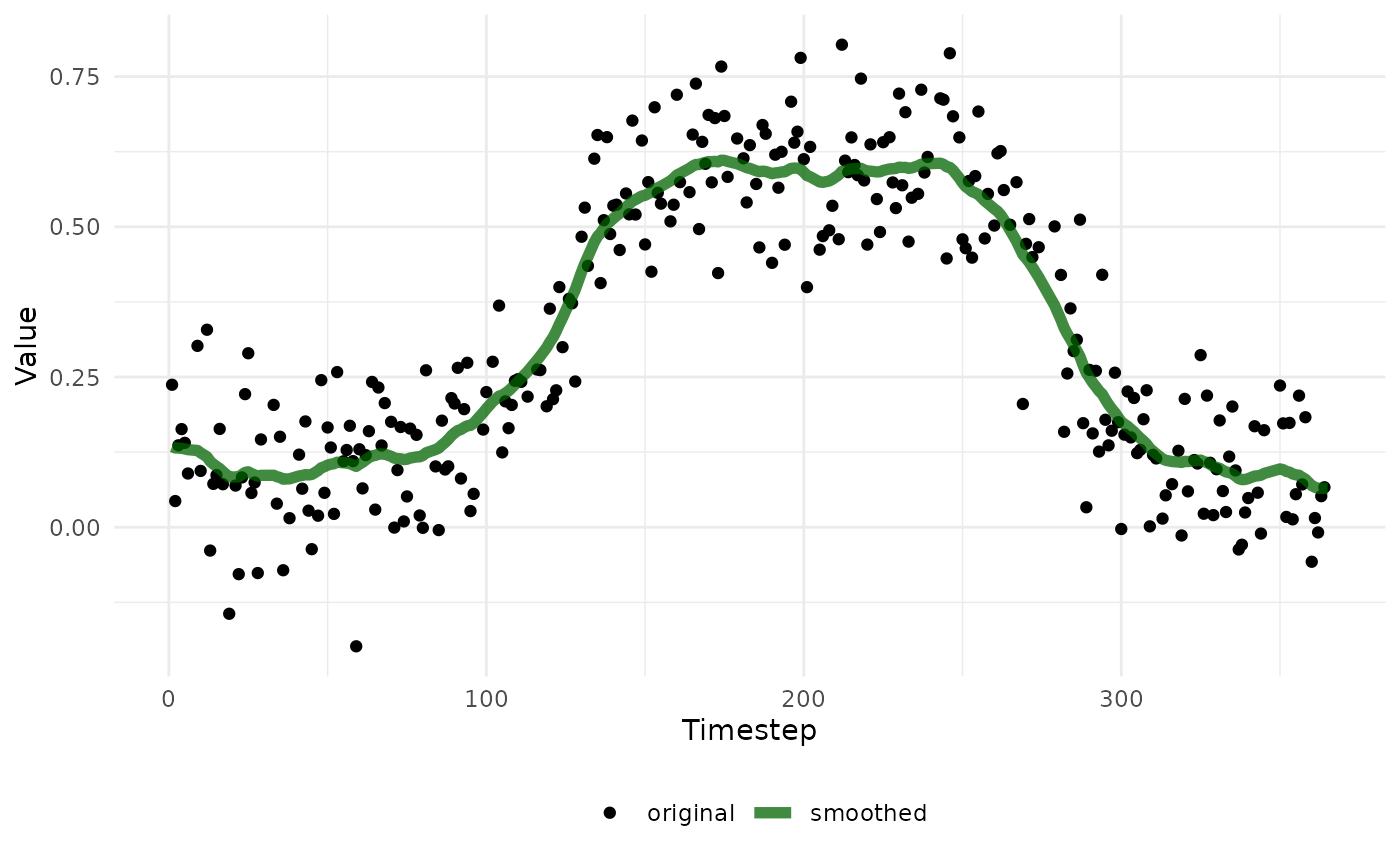

Determine seasonality

The determine_seasonality() function is used to check if a time series from one year (or one life cycle) has seasonal variations or has no significant variations. In practice, we can use this function to distinguish if the greenness of a tree within a year has seasonal variations (e.g., deciduous trees) or remains relatively constant (e.g., evergreen trees). Under the hood, the function fits a simple linear regression model and segmented regression models with 1 to 3 breakpoints to a given time series. It then compares their Akaike Information Criterion (AIC) values (with a penalty parameter k) to assess whether a simple linear regression (i.e., non-segmented) model is preferred. The k parameter controls the penalty for the number of breakpoints in the calculation of AIC. A larger k means that the favored model is more likely to be a simple linear regression model, such that we are more conservative in concluding that the time series has seasonal variations.

# Check if a time series is flat
example_seasonality <- determine_seasonality(
  ts = simulate_ts,
  k = 50
)

print(stringr::str_c("Time series has significant seasonal variation: ", example_seasonality))

## [1] "Time series has significant seasonal variation: TRUE"

Yiluan Song

2026-03-05

Gap-filling and smoothing

Determine seasonality