Preprocess data

dat_shoot_alive <- dat_shoot %>%
  drop_na(barcode) %>%
  filter(shoot > 0) %>%
  filter(!is.na(shoot)) %>%
  group_by(barcode, year) %>%
  mutate(shoot_alive = if_else(any(alive == 0), 0, 1)) %>% # filter out plants ever considered dead at any point in a year
  ungroup() %>%
  filter(shoot_alive == 1) %>%
  select(-alive, -shoot_alive)

dat_all <- dat_shoot_alive %>%
  mutate(model = str_c(species, canopy, water_name, sep = "_")) %>%
  group_by(species, model) %>%
  mutate(individual = str_c(barcode, year, sep = "_") %>% factor() %>% as.integer()) %>% # individual level random effects)
  mutate(group = str_c(site, year, sep = "_") %>% factor() %>% as.integer()) %>% # site-year level random effects
  ungroup() %>%
  tidy_treatment_code()

df_onoff <- dat_climate_daily %>%
  group_by(site, block, year) %>%
  filter(heat_onoff == "on") %>%
  summarise(
    first_on = min(doy),
    last_on = max(doy)
  ) %>%
  arrange(year, site, block) %>%
  group_by(year) %>%
  summarise(
    first_on = max(first_on),
    last_on = min(last_on)
  ) %>%
  filter(year != 2012) %>% # 2012 is an incomplete year
  mutate(
    firston_date = lubridate::date(paste0(year, "-01-01")) + (first_on - 1),
    last_on_date = lubridate::date(paste0(year, "-01-01")) + (last_on - 1)
  )

ls_dat_climate_gs <- list()
for (i in 1:nrow(df_onoff)) {
  ls_dat_climate_gs[[i]] <- summ_climate_season(
    dat_climate_daily %>% filter(year == df_onoff$year[i]),
    doy_start = df_onoff$first_on[i],
    doy_end = df_onoff$last_on[i],
    rainfall = 1,
    group_vars = c("site", "block", "plot", "canopy", "heat", "heat_name", "water", "water_name", "year")
  )
}
dat_climate_gs <- ls_dat_climate_gs %>% bind_rows()

dat_climate_gs_ambient <- calc_climate_ambient(dat_climate = dat_climate_gs, dat_shoot)
dat_climate_gs_diff <- calc_climate_diff(dat_climate = dat_climate_gs, dat_climate_ambient = dat_climate_gs_ambient)

dat_all_cov <- dat_all %>%
  left_join(dat_climate_gs_diff %>%
    group_by(site, canopy, heat, water) %>%
    summarise(delta_temp = mean(delta_temp, na.rm = T), delta_mois = mean(delta_mois, na.rm = T)) %>%
    mutate(
      delta_temp = if_else(heat == "_", 0, delta_temp),
      delta_mois = if_else(heat == "_", 0, delta_mois)
    ))

Shoot growth model

Data model

\[\begin{align*} log(y_{j,t,s,d}) \sim \text{Normal}(\mu_{j,t,s,d}, \sigma^2) \end{align*}\]

Process model

\[\begin{align*} \mu_{j,t,s,d} &= c+\frac{A_{j,t,s}}{1+e^{-k_{j,t,s}(d-x_{0 j,t,s})}} \newline A_{j,t,s} &\sim \text{Normal} (\mu_A + \delta_{A,j}+ \alpha_{A,t,s}, \tau_A^2) \newline x_{0 j,t,s} &\sim \text{Normal} (\mu_{x_0} + \delta_{x_0,i}+ \alpha_{x_0,t,s}, \tau_{x_0}^2) \newline log(k_{j,t,s}) &\sim \text{Normal} (\mu_{log(k)} + \delta_{log(k),i}+ \alpha_{log(k),t,s}, \tau_{log(k)}^2) \end{align*}\]

Fixed effects

\[\begin{align*} \delta_{A,j} &= \beta_{A} W_j \newline \delta_{x_0,j} &= \beta_{x_0} W_j \newline \delta_{log(k),j} &= \beta_{log(k)} W_j \end{align*}\]

Random effects

\[\begin{align*} \alpha_{A,t,s} &\sim \text{Normal}(0, \sigma_A^2) \newline \alpha_{x_0,t,s} &\sim \text{Normal}(0, \sigma_{x_0}^2) \newline \alpha_{log(k),t,s} &\sim \text{Normal}(0, \sigma_{log(k)}^2) \end{align*}\]

Priors

\[\begin{align*} c &\sim \text{Uniform}(0, 3) \newline \mu_A &\sim \text{Uniform}(1, 6) \newline \beta_A &\sim \text{Normal} (0,0.5)\newline \tau_A &\sim \text{Truncated Normal}(0, 0.25, 0, \infty) \newline \sigma_A &\sim \text{Truncated Normal}(0, 0.5, 0, \infty) \newline \mu_{x_0} &\sim \text{Uniform}(120, 180) \newline \beta_{x_0} &\sim \text{Normal} (0,5)\newline \tau_{x_0} &\sim \text{Truncated Normal}(0, 2.5, 0, \infty) \newline \sigma_{x_0} &\sim \text{Truncated Normal}(0, 5, 0, \infty) \newline \mu_{log(k)} &\sim \text{Uniform}(-3.5, -1) \newline \beta_{log(k)} &\sim \text{Normal} (0,0.1)\newline \tau_{log(k)} &\sim \text{Truncated Normal}(0, 0.05, 0, \infty) \newline \sigma_{log(k)}^2 &\sim \text{Truncated Normal}(0, 0.1, 0, \infty) \newline \sigma^2 &\sim \text{Truncated Normal}(0, 1, 0, \infty) \end{align*}\]

Fit model

calc_bayes_all(
  data = dat_all_cov,
  independent_priors = F, # do not use species-specific empirical informative priors
  uniform_priors = T, # use uniform priors
  intui_param = F, # regular parameterization with asym, xmid, logk
  continuous_cov = T, # continuous covariates
  individual_trajectory = T, # individual level random effects
  num_iterations = 50000,
  nthin = 5,
  path = "alldata/intermediate/shootmodeling/individual_continuous/",
  num_cores = 35
)
calc_bayes_derived(path = "alldata/intermediate/shootmodeling/individual_continuous/", num_cores = 35, random = T, random_fast = T)
plot_bayes_all(path = "alldata/intermediate/shootmodeling/individual_continuous/", continuous_cov = T, num_cores = 35)

MCMC

df_bayes_all <- read_bayes_all(path = "alldata/intermediate/shootmodeling/individual_continuous/", full_factorial = F, derived = F, tidy_mcmc = F)

p_bayes_diagnostics <- plot_bayes_diagnostics(df_MCMC = df_bayes_all %>% filter(model == "aceru_open_ambient"), plot_corr = F)
p_bayes_diagnostics$p_MCMC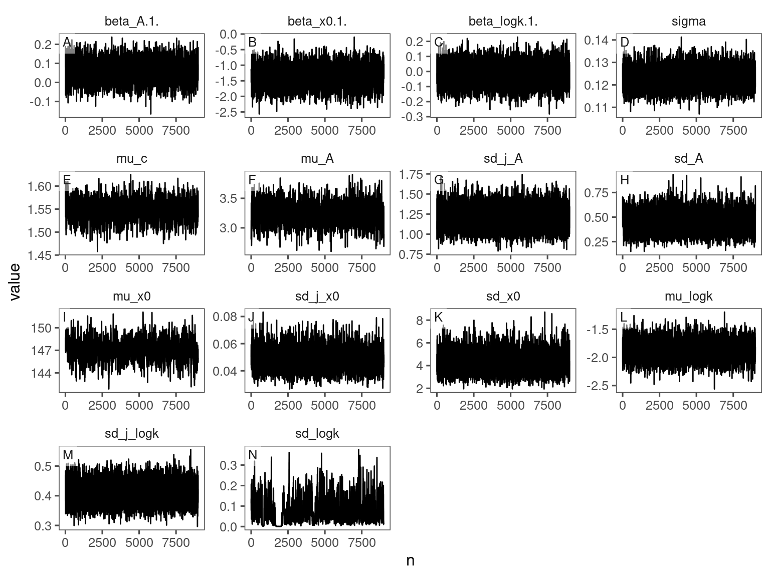

p_bayes_diagnostics$p_posterior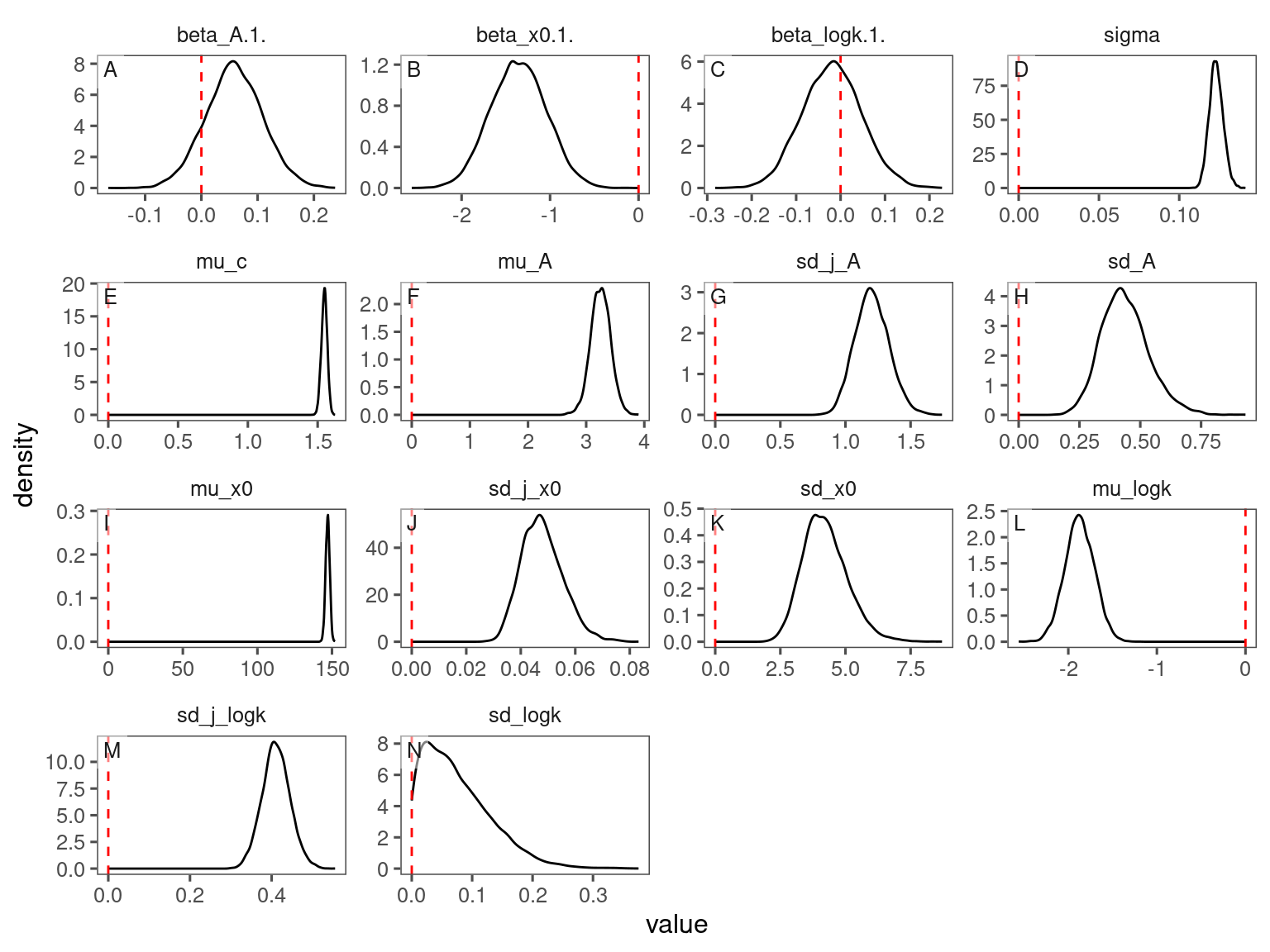

Conditional predictions

df_bayes_pred_all <- read_bayes_all(path = "alldata/intermediate/shootmodeling/individual_continuous/", full_factorial = F, content = "predict")

p_bayes_predict <- plot_bayes_predict(
  data = dat_all %>% filter(species == "aceru") %>% filter(shoot > exp(-1)),
  data_predict = df_bayes_pred_all %>% filter(str_detect(model, "aceru")) %>% filter(pred_median > exp(-1)),
  vis_log = T,
  vis_ci = F
)

p_bayes_predict$p_overlay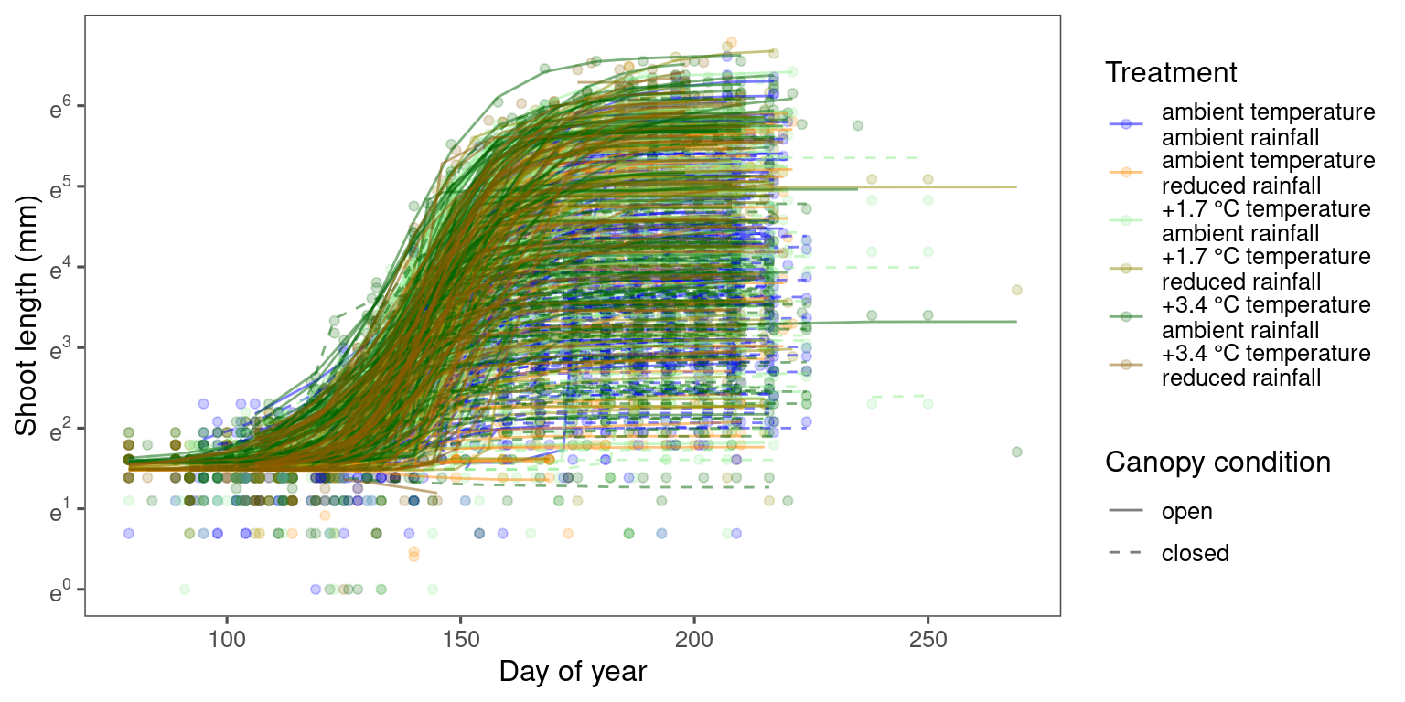

Accuracy

p_bayes_predict$p_accuracy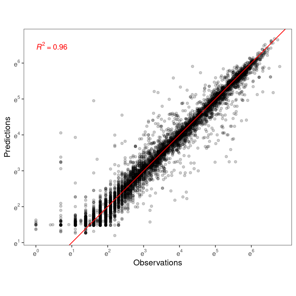

Marginal predictions

df_bayes_pred_marginal_all <- read_bayes_all(path = "alldata/intermediate/shootmodeling/individual_continuous/", full_factorial = F, content = "predict_marginal")

p_bayes_predict <- plot_bayes_predict(
  data_predict = df_bayes_pred_marginal_all %>% filter(str_detect(model, "aceru")),
  vis_log = T,
  vis_ci = F,
  continuous_cov = T,
  marginal = T
)
p_bayes_predict$p_predict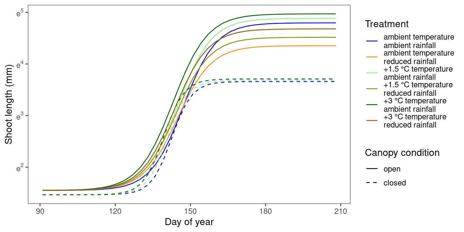

Coefficients

Read in summary of inferred parameters

v_species <- read_species() %>%
  select(species = acronym, species_type, origin) %>%
  left_join(read_trait_niche()) %>%
  arrange(species_type, desc(origin), temperature_niche) %>%
  pull(species)

df_bayes_mcmc <- read_bayes_all(path = "alldata/intermediate/shootmodeling/individual_continuous/", full_factorial = F, derived = T, tidy_mcmc = T, content = "mcmc")

df_mcmc <- df_bayes_mcmc %>%
  tidy_species_name(species_order = v_species) %>%
  tidy_model_name()

df_shoot_coef <- df_bayes_mcmc %>%
  summ_mcmc(option = "all", stats = "median") %>%
  tidy_species_name(species_order = v_species) %>%
  tidy_model_name()

df_shoot_mu <- df_bayes_mcmc %>%
  summ_mcmc(option = "mu", stats = "median") %>%
  tidy_species_name(species_order = v_species) %>%
  tidy_model_name()

p_bayes_summ <- plot_bayes_summary(df_mcmc %>% filter(response %in% c("start", "total growth", "duration", "speed")), option = "coef", derived_metric = "all", stack = T, symmetric = T)$p_coef_line +
  tagger::tag_facets(
    tag_prefix = "A", tag_suffix = "",
    tag_pool = patch_tagger(ncol = 2, npanel = 4, tag_level = "1", option = "wrap")
  )

p_coef_2group <- plot_response_trait(df_shoot_coef, df_shoot_mu = df_shoot_mu, x_var = "species_type", y_var = c("start", "total growth", "duration", "speed"), y_type = "response", species_name = F, empirical = T, points = T, group_summary = T, anova = T, symmetric = T) +
  scale_x_discrete(labels = function(x) str_replace(x, " ", "\n")) +
  tagger::tag_facets(
    tag_prefix = "B", tag_suffix = "",
    tag_pool = patch_tagger(ncol = 2, npanel = 4, tag_level = "1", option = "wrap")
  ) +
  theme(legend.position = "bottom")

wrap_elements(p_bayes_summ) + wrap_elements(p_coef_2group) +
  plot_layout(
    ncol = 1
  ) &
  theme(tagger.panel.tag.background = element_blank()) + theme(tagger.panel.tag.background = element_rect(fill = NA))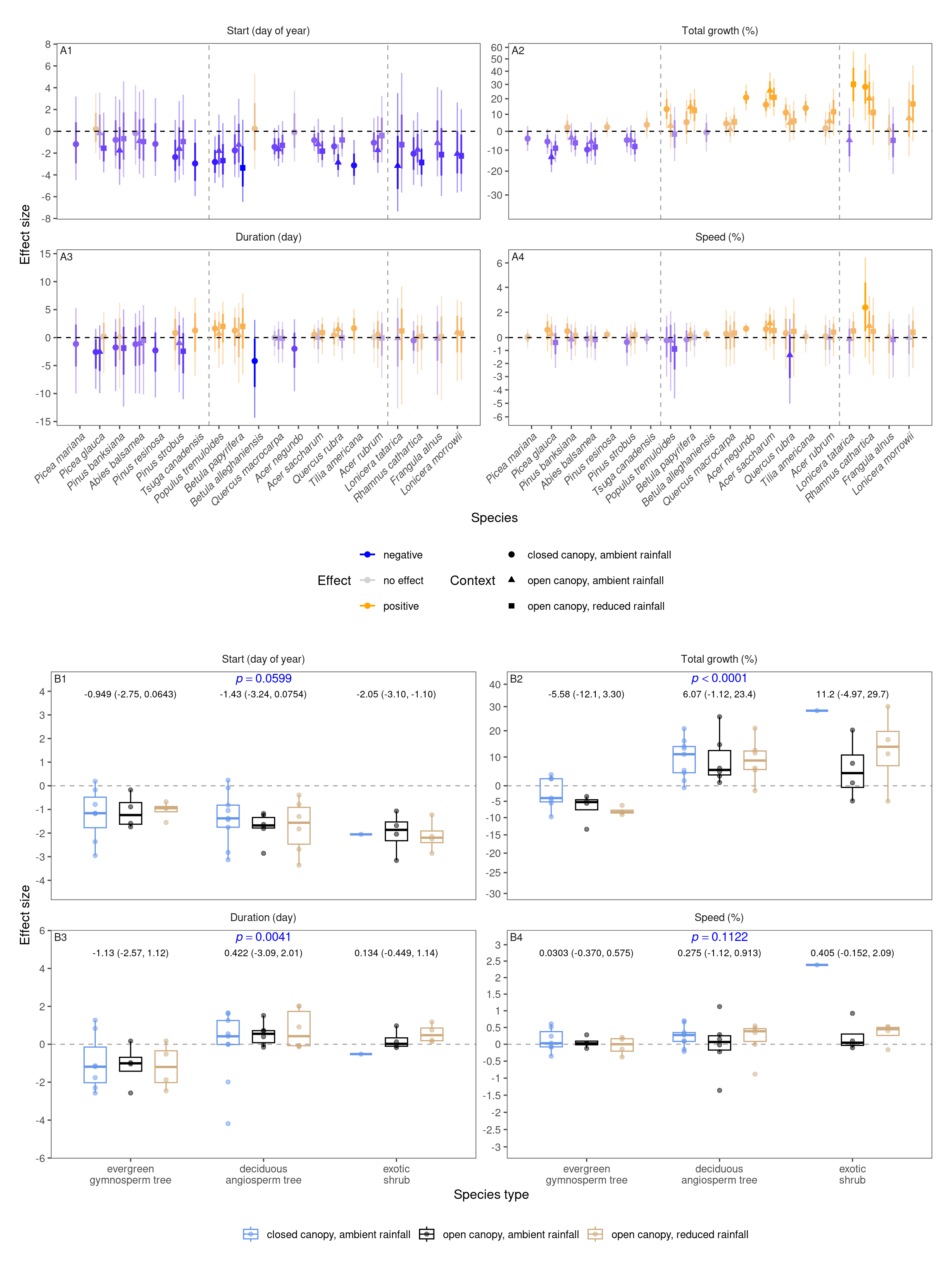

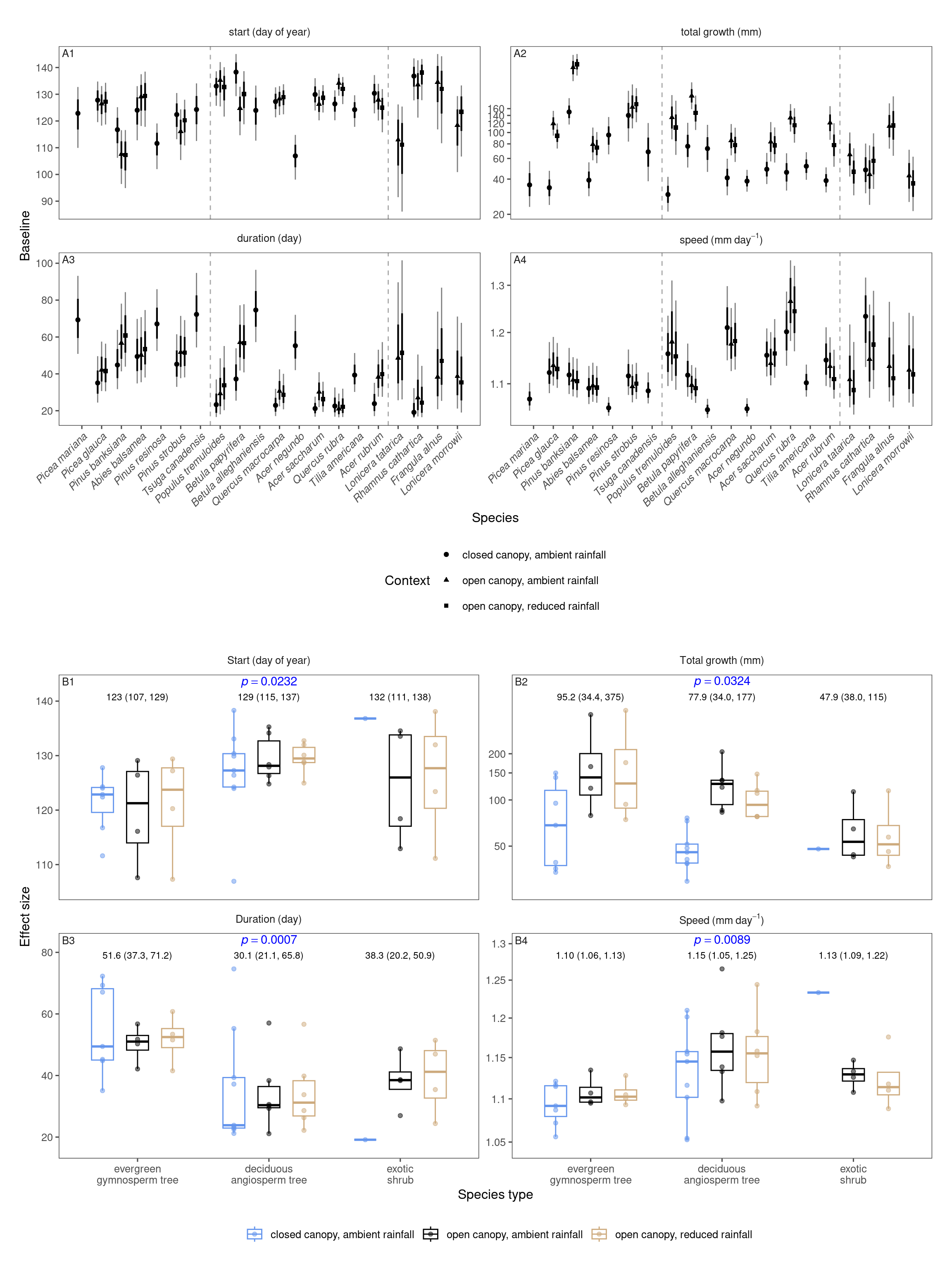
Baseline

p_bayes_summ <- plot_bayes_summary(df_mcmc %>% filter(response %in% c("start", "total growth", "duration", "speed")), option = "mu", derived_metric = "all", stack = T)$p_coef_line +
  tagger::tag_facets(
    tag_prefix = "A", tag_suffix = "",
    tag_pool = patch_tagger(ncol = 2, npanel = 4, tag_level = "1", option = "wrap")
  )

p_coef_2group <- plot_response_trait(df_shoot_coef, df_shoot_mu = df_shoot_mu, x_var = "species_type", y_var = c("start", "total growth", "duration", "speed"), y_type = "baseline", species_name = F, empirical = T, points = T, group_summary = T, anova = T) +
  scale_x_discrete(labels = function(x) str_replace(x, " ", "\n")) +
  tagger::tag_facets(
    tag_prefix = "B", tag_suffix = "",
    tag_pool = patch_tagger(ncol = 2, npanel = 4, tag_level = "1", option = "wrap")
  ) +
  theme(legend.position = "bottom")

wrap_elements(p_bayes_summ) + wrap_elements(p_coef_2group) +
  plot_layout(
    ncol = 1
  ) &
  theme(tagger.panel.tag.background = element_blank()) + theme(tagger.panel.tag.background = element_rect(fill = NA))

Continuous predictors to replace warming treatment

Preprocess data

Shoot growth model

Fit model

Coefficients