In the previous hierarchical Bayesian model, I pooled data at the site-year level, meaning that all individual plants from the same species, warming treatment, drying treatment, canopy condition, site, and year contributed to estimating a single trajectory. This complete pooling did help to average out individual-level noise, but it has a few drawbacks.
A growth curve through data points from all individuals is not the same as a growth curve of a typical or average individual. (Jensen’s inequality.) If we assume that each individual has a logistic growth curve, then the average of many logistic curves is usually not a logistic curve.
It gave different inferences compared to the two-stage frequentist approach (NLS-LME). The discrepancy between population and individual levels might be a possible reason.
It might be more prone to missing data problems. Some individuals that were only measured in part of the trajectory might bias the population-level trajectory.
It ignores individual-level variations in growth and phenological parameters, which were substantial.
Therefore, in this version, we assume that each individual has its own trajectory, and the individual-level parameters are drawn from distributions centered around population-level parameters.
If this hierarchical Bayesian approach works, it should be better than the two-step frequentist approach, because: 1. It can borrow strength across individuals’ and’ partial trajectories to estimate parameters more accurately. 2. It can account for uncertainty in individual-level parameters when estimating population-level parameters.
Pre-process data
dat_shoot_alive <- dat_shoot %>%
  drop_na(barcode) %>%
  filter(shoot > 0) %>%
  filter(!is.na(shoot)) %>%
  group_by(barcode, year) %>%
  mutate(shoot_alive = if_else(any(alive == 0), 0, 1)) %>% # filter out plants ever considered dead at any point in a year
  ungroup() %>%
  filter(shoot_alive == 1) %>%
  select(-alive, -shoot_alive)

dat_all <- dat_shoot_alive %>%
  mutate(model = str_c(species, canopy, water_name, sep = "_")) %>%
  group_by(species, model) %>%
  mutate(individual = str_c(barcode, year, sep = "_") %>% factor() %>% as.integer()) %>% # individual level random effects)
  mutate(group = str_c(site, year, sep = "_") %>% factor() %>% as.integer()) %>% # site-year level random effects
  ungroup() %>%
  tidy_treatment_code()
Shoot growth model
Data model
\[\begin{align*} log(y_{j,t,s,d}) \sim \text{Normal}(\mu_{j,t,s,d}, \sigma^2) \end{align*}\]
Process model
\[\begin{align*} \mu_{j,t,s,d} &= c+\frac{A_{j,t,s}}{1+e^{-k_{j,t,s}(d-x_{0 j,t,s})}} \newline A_{j,t,s} &\sim \text{Normal} (\mu_A + \delta_{A,j}+ \alpha_{A,t,s}, \tau_A^2) \newline x_{0 j,t,s} &\sim \text{Normal} (\mu_{x_0} + \delta_{x_0,i}+ \alpha_{x_0,t,s}, \tau_{x_0}^2) \newline log(k_{j,t,s}) &\sim \text{Normal} (\mu_{log(k)} + \delta_{log(k),i}+ \alpha_{log(k),t,s}, \tau_{log(k)}^2) \end{align*}\]
Fixed effects
\[\begin{align*} \delta_{A,j} &= \beta_{A} W_j \newline \delta_{x_0,j} &= \beta_{x_0} W_j \newline \delta_{log(k),j} &= \beta_{log(k)} W_j \end{align*}\]
Random effects
\[\begin{align*} \alpha_{A,t,s} &\sim \text{Normal}(0, \sigma_A^2) \newline \alpha_{x_0,t,s} &\sim \text{Normal}(0, \sigma_{x_0}^2) \newline \alpha_{log(k),t,s} &\sim \text{Normal}(0, \sigma_{log(k)}^2) \end{align*}\]
Priors
\[\begin{align*} c &\sim \text{Uniform}(0, 3) \newline \mu_A &\sim \text{Uniform}(1, 6) \newline \beta_A &\sim \text{Normal} (0,0.5)\newline \tau_A &\sim \text{Truncated Normal}(0, 0.25, 0, \infty) \newline \sigma_A &\sim \text{Truncated Normal}(0, 0.5, 0, \infty) \newline \mu_{x_0} &\sim \text{Uniform}(120, 180) \newline \beta_{x_0} &\sim \text{Normal} (0,5)\newline \tau_{x_0} &\sim \text{Truncated Normal}(0, 2.5, 0, \infty) \newline \sigma_{x_0} &\sim \text{Truncated Normal}(0, 5, 0, \infty) \newline \mu_{log(k)} &\sim \text{Uniform}(-3.5, 0) \newline \beta_{log(k)} &\sim \text{Normal} (0,0.1)\newline \tau_{log(k)} &\sim \text{Truncated Normal}(0, 0.05, 0, \infty) \newline \sigma_{log(k)}^2 &\sim \text{Truncated Normal}(0, 0.1, 0, \infty) \newline \sigma^2 &\sim \text{Truncated Normal}(0, 1, 0, \infty) \end{align*}\]
This time, I tightened the priors a bit because of poptr and betpa had large variability but lacked data after using separate models. I had to impose stronger regularization to reduce the risk of overfitting.
Fit model
calc_bayes_all(
  data = dat_all,
  independent_priors = F, # do not use species-specific empirical informative priors
  uniform_priors = T, # use uniform priors
  intui_param = F, # regular parameterization with asym, xmid, logk
  individual_trajectory = T, # individual level random effects
  num_iterations = 50000,
  nthin = 5,
  path = "alldata/intermediate/shootmodeling/individual/",
  num_cores = 35
)
calc_bayes_derived(path = "alldata/intermediate/shootmodeling/individual/", num_cores = 35, random = T, random_fast = T)
plot_bayes_all(path = "alldata/intermediate/shootmodeling/individual/", num_cores = 35)
MCMC
df_bayes_all <- read_bayes_all(path = "alldata/intermediate/shootmodeling/individual/", full_factorial = F, derived = F, tidy_mcmc = F)p_bayes_diagnostics <- plot_bayes_diagnostics(df_MCMC = df_bayes_all %>% filter(model == "aceru_open_ambient"), plot_corr = F)
p_bayes_diagnostics$p_MCMC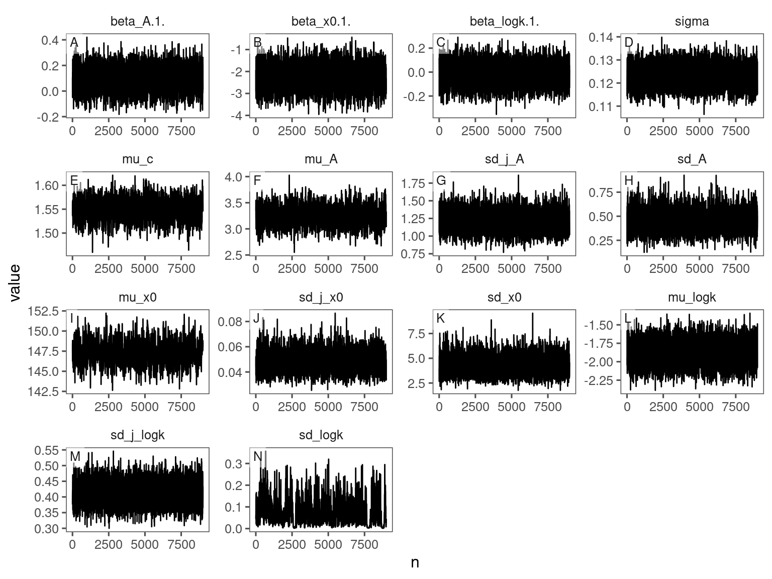
p_bayes_diagnostics$p_posterior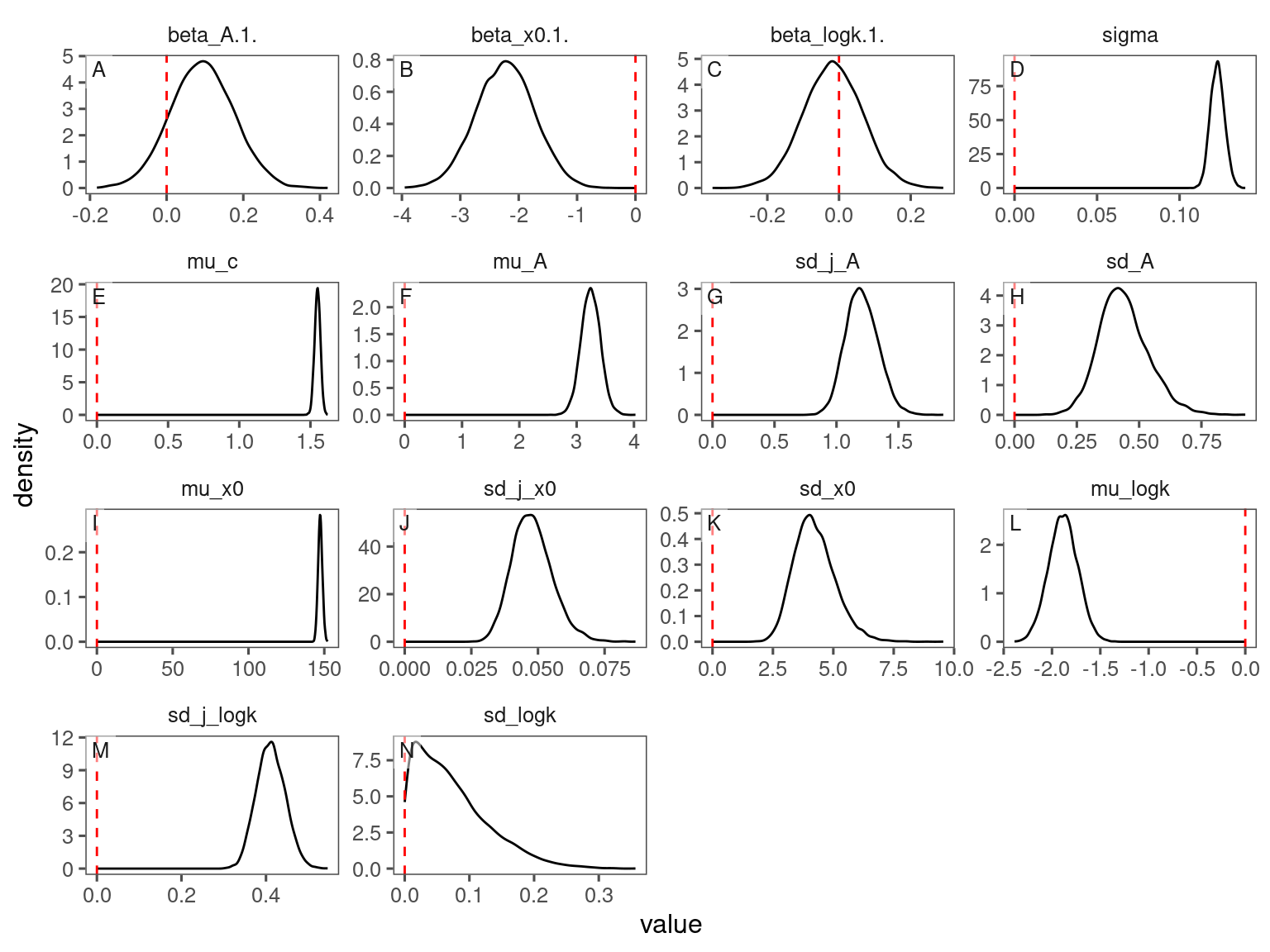
Conditional predictions
df_bayes_pred_all <- read_bayes_all(path = "alldata/intermediate/shootmodeling/individual/", full_factorial = F, content = "predict")

p_bayes_predict <- plot_bayes_predict(
  data = dat_all %>% filter(species == "aceru") %>% filter(shoot >= exp(-1)),
  data_predict = df_bayes_pred_all %>% filter(str_detect(model, "aceru")) %>% filter(pred_median >= exp(-1)),
  vis_log = T,
  vis_ci = F
)

p_bayes_predict$p_overlay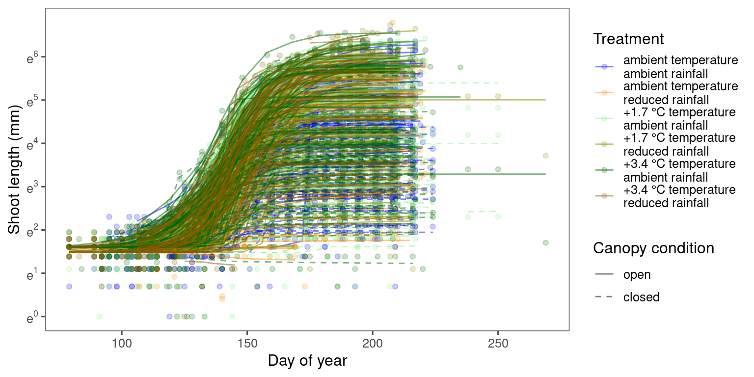
Accuracy
p_bayes_predict$p_accuracy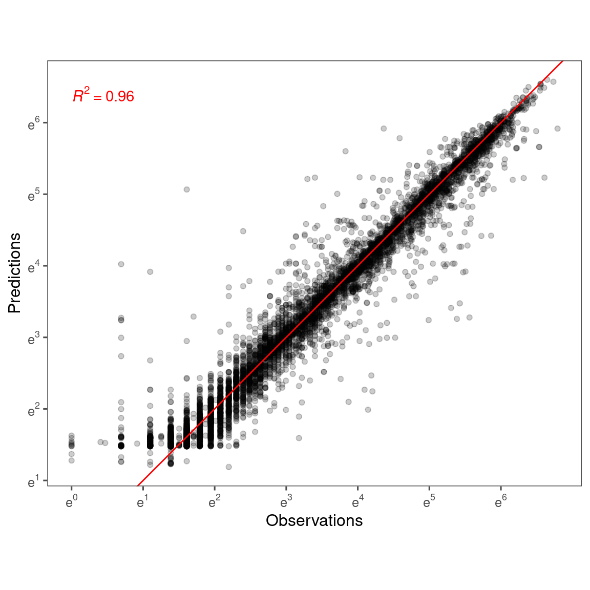
Marginal predictions
df_bayes_pred_marginal_all <- read_bayes_all(path = "alldata/intermediate/shootmodeling/individual/", full_factorial = F, content = "predict_marginal")

p_bayes_predict <- plot_bayes_predict(
  data_predict = df_bayes_pred_marginal_all %>% filter(str_detect(model, "aceru")),
  vis_log = T,
  vis_ci = F
)
p_bayes_predict$p_predict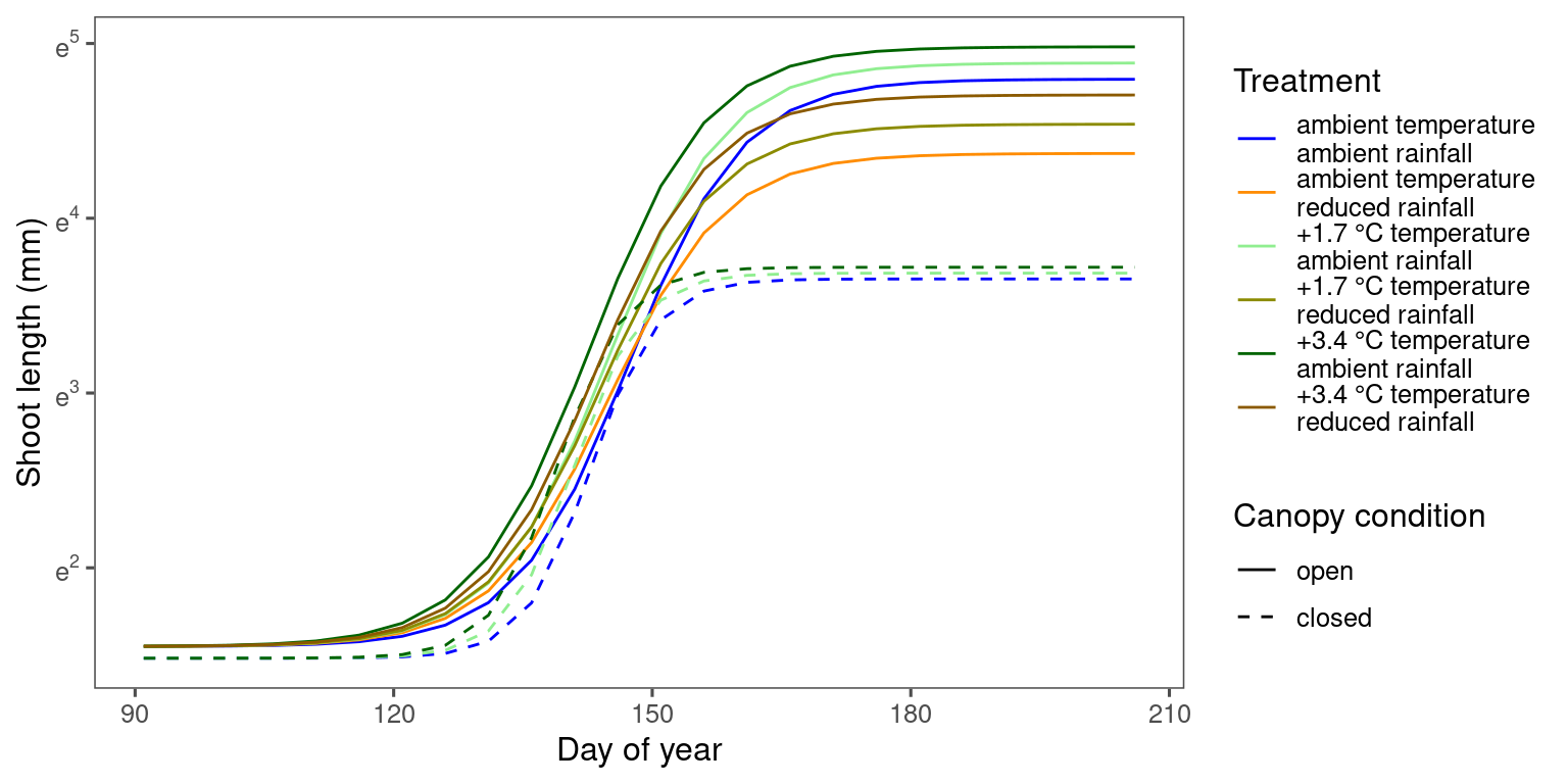
Coefficients
Read in summary of inferred parameters
v_species <- read_species() %>%
  select(species = acronym, species_type, origin) %>%
  left_join(read_trait_niche()) %>%
  arrange(species_type, desc(origin), temperature_niche) %>%
  pull(species)

df_bayes_mcmc <- read_bayes_all(path = "alldata/intermediate/shootmodeling/individual/", full_factorial = F, derived = T, tidy_mcmc = T, content = "mcmc")

df_mcmc <- df_bayes_mcmc %>%
  tidy_species_name(species_order = v_species) %>%
  tidy_model_name() %>%
  mutate(value = value * (str_detect(param, "beta") + 1)) # effect of 3.4 degree C warming instead of 1.7 degree C

df_shoot_coef <- df_bayes_mcmc %>%
  mutate(value = value * (str_detect(param, "beta") + 1)) %>% # effect of 3.4 degree C warming instead of 1.7 degree C
  summ_mcmc(option = "all", stats = "median") %>%
  tidy_species_name(species_order = v_species) %>%
  tidy_model_name()

df_shoot_mu <- df_bayes_mcmc %>%
  summ_mcmc(option = "mu", stats = "median") %>%
  tidy_species_name(species_order = v_species) %>%
  tidy_model_name()
p_bayes_summ <- plot_bayes_summary(df_mcmc %>% filter(response %in% c("start", "total growth", "duration", "speed")), option = "coef", derived_metric = "all", stack = T)$p_coef_line +
tagger::tag_facets(
tag_prefix = "A", tag_suffix = "",
tag_pool = patch_tagger(ncol = 2, npanel = 4, tag_level = "1", option = "wrap")
)p_coef_2group <- plot_response_trait(df_shoot_coef, df_shoot_mu = df_shoot_mu, x_var = "species_type", y_var = c("start", "total growth", "duration", "speed"), y_type = "response", species_name = F, empirical = T, points = T, group_summary = T, anova = T) +
scale_x_discrete(labels = function(x) str_replace(x, " ", "\n")) +
tagger::tag_facets(
tag_prefix = "B", tag_suffix = "",
tag_pool = patch_tagger(ncol = 2, npanel = 4, tag_level = "1", option = "wrap")
) +
theme(legend.position = "bottom")wrap_elements(p_bayes_summ) + wrap_elements(p_coef_2group) +
plot_layout(
ncol = 1
) &
theme(tagger.panel.tag.background = element_blank()) + theme(tagger.panel.tag.background = element_rect(fill = NA))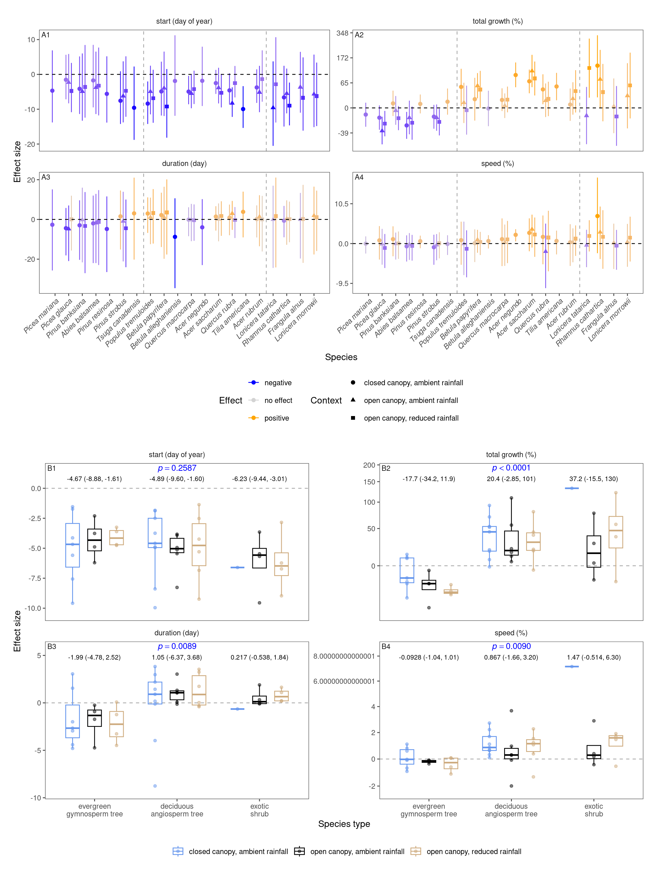
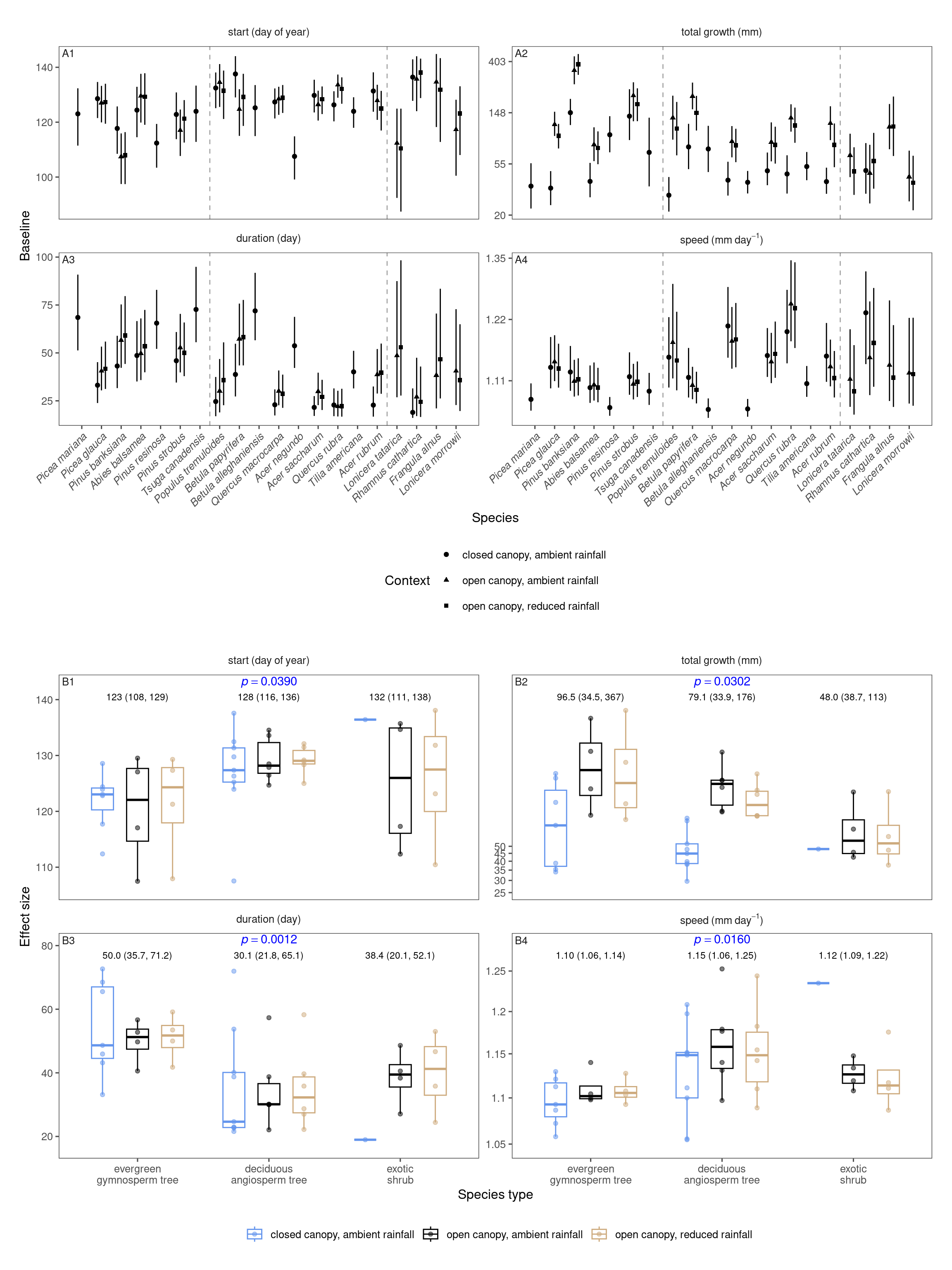
Baseline
p_bayes_summ <- plot_bayes_summary(df_mcmc %>% filter(response %in% c("start", "total growth", "duration", "speed")), option = "mu", derived_metric = "all", stack = T)$p_coef_line +
  tagger::tag_facets(
    tag_prefix = "A", tag_suffix = "",
    tag_pool = patch_tagger(ncol = 2, npanel = 4, tag_level = "1", option = "wrap")
  )
p_coef_2group <- plot_response_trait(df_shoot_coef, df_shoot_mu = df_shoot_mu, x_var = "species_type", y_var = c("start", "total growth", "duration", "speed"), y_type = "baseline", species_name = F, empirical = T, points = T, group_summary = T, anova = T) +
scale_x_discrete(labels = function(x) str_replace(x, " ", "\n")) +
tagger::tag_facets(
tag_prefix = "B", tag_suffix = "",
tag_pool = patch_tagger(ncol = 2, npanel = 4, tag_level = "1", option = "wrap")
) +
theme(legend.position = "bottom")wrap_elements(p_bayes_summ) + wrap_elements(p_coef_2group) +
plot_layout(
ncol = 1
) &
theme(tagger.panel.tag.background = element_blank()) + theme(tagger.panel.tag.background = element_rect(fill = NA))