Forecasting with experiment: Shoot (total growth)

Visualize differences between treatments

dat_shoot_alive <- dat_shoot %>%
  drop_na(barcode) %>%
  filter(shoot > 0) %>%
  drop_na(shoot) %>%
  group_by(barcode, year) %>%
  mutate(shoot_alive = if_else(any(alive == 0), 0, 1)) %>% # filter out plants ever considered dead at any point in a year
  ungroup() %>%
  filter(shoot_alive == 1) %>%
  select(-alive, -shoot_alive)

df_param_all <- calc_empirical_parameters(df = dat_shoot_alive, path = "alldata/intermediate/", log = T, overwrite = F) %>%
  tidy_species_name()

df_param_diff <- calc_parameter_diff(df_param_all)

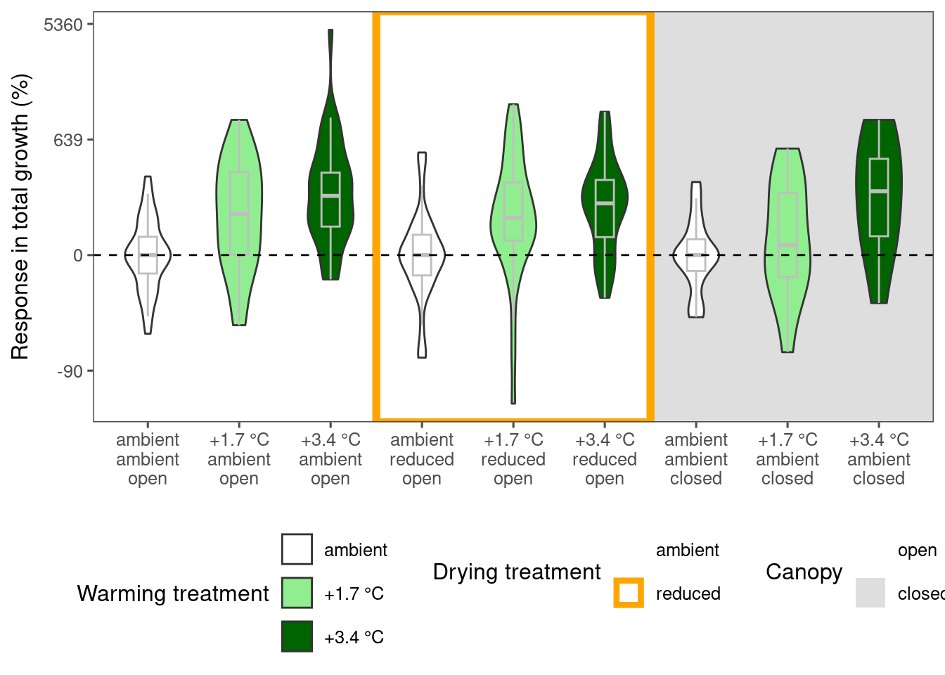
plot_metric_difference(
  dat_diff = df_param_diff %>%
    filter(
      species %in% c("acesa"),
      param %in% c("total growth")
    ), type = "shoot", x_label_short = F, simple = F
)

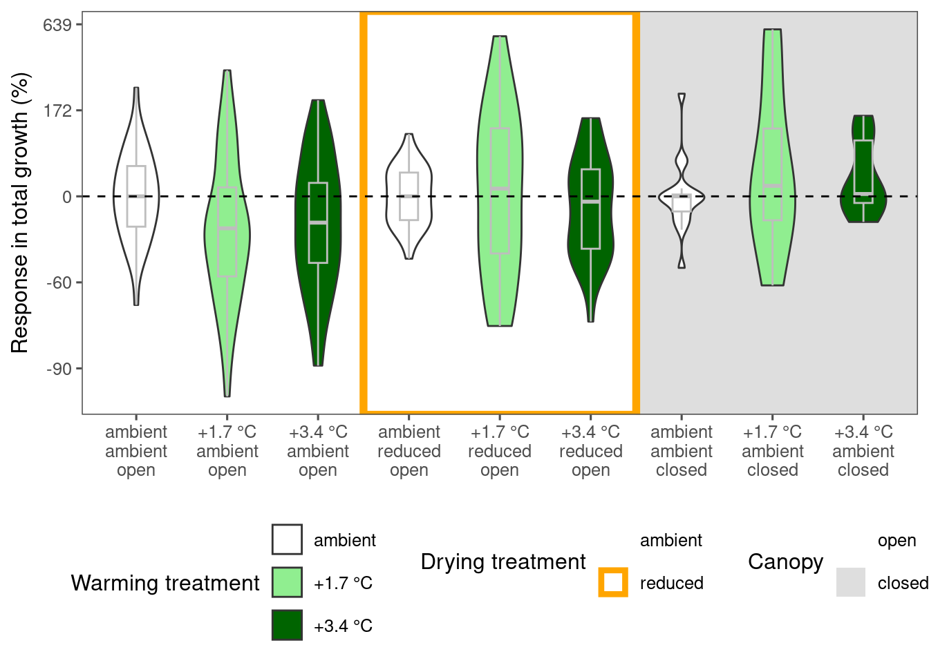
plot_metric_difference(
  dat_diff = df_param_diff %>%
    filter(
      species %in% c("picgl"),
      param %in% c("total growth")
    ), type = "shoot", x_label_short = F, simple = F
)

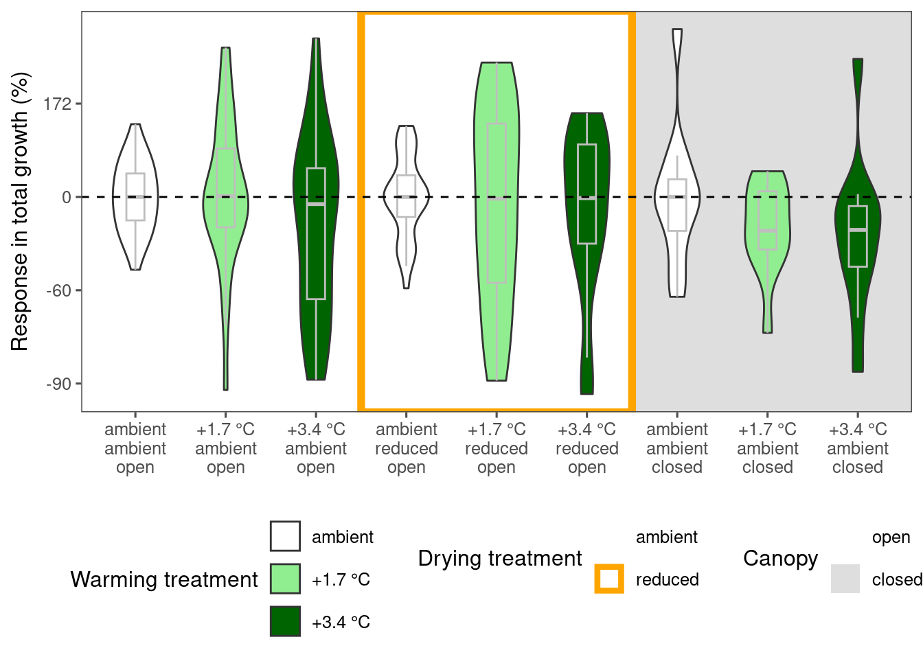
plot_metric_difference(
  dat_diff = df_param_diff %>%
    filter(
      species %in% c("abiba"),
      param %in% c("total growth")
    ), type = "shoot", x_label_short = F, simple = F
)

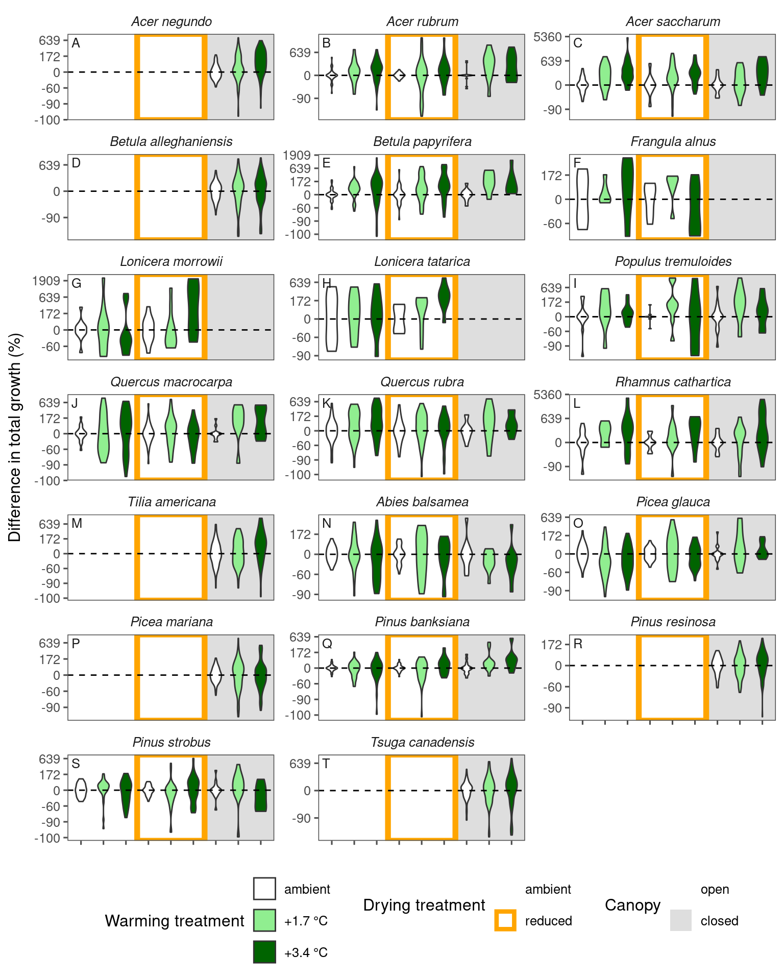
plot_metric_difference(
  dat_diff = df_param_diff %>%
    filter(param %in% c("total growth")), type = "shoot", x_label_short = T, simple = T
)

Visualize observational trends

dat_climate_spring <- summ_climate_season(dat_climate_daily, date_start = "Mar 15", date_end = "May 15", rainfall = 1, group_vars = c("site", "block", "plot", "canopy", "heat", "heat_name", "water", "water_name", "year"))

plot_observational_trend(df_param_all %>% filter(species %in% c("acesa"), param == "total growth"), dat_climate_spring, type = "shoot")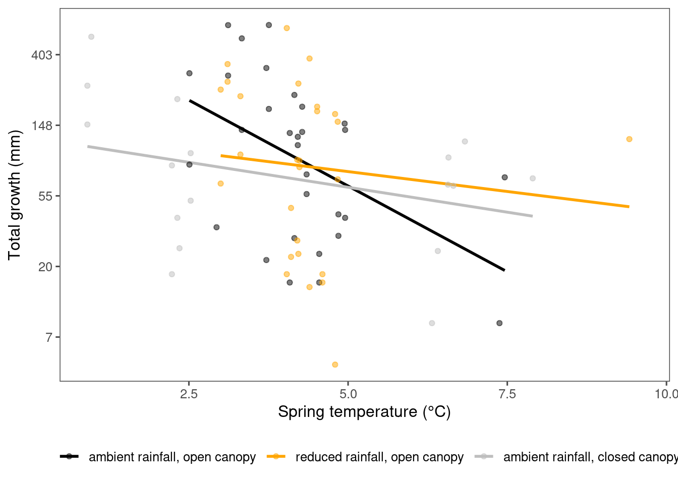

plot_observational_trend(df_param_all %>% filter(species %in% c("picgl"), param == "total growth"), dat_climate_spring, type = "shoot")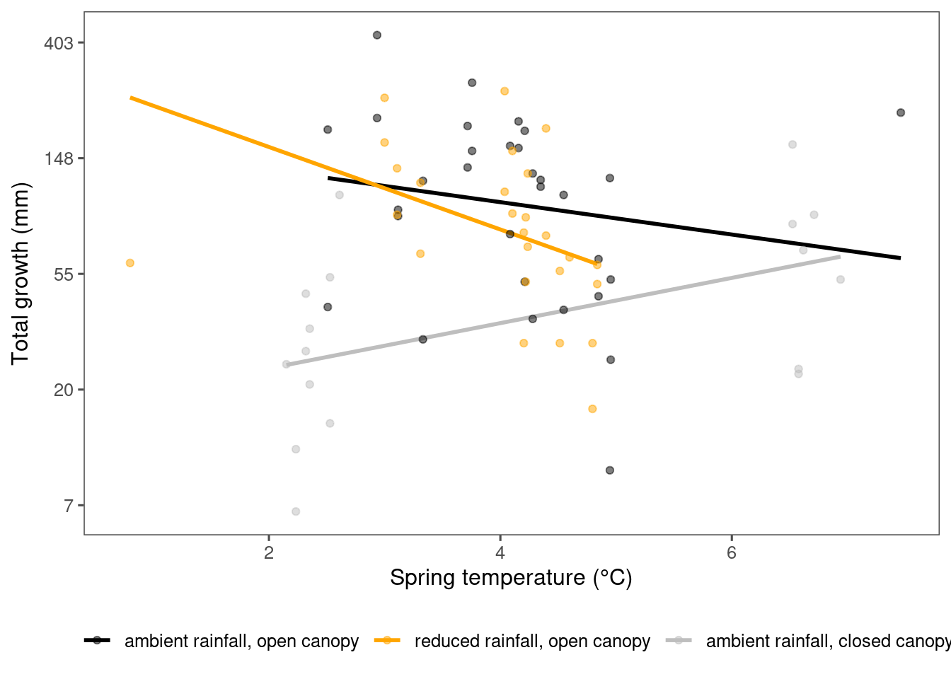

plot_observational_trend(df_param_all %>% filter(species %in% c("abiba"), param == "total growth"), dat_climate_spring, type = "shoot")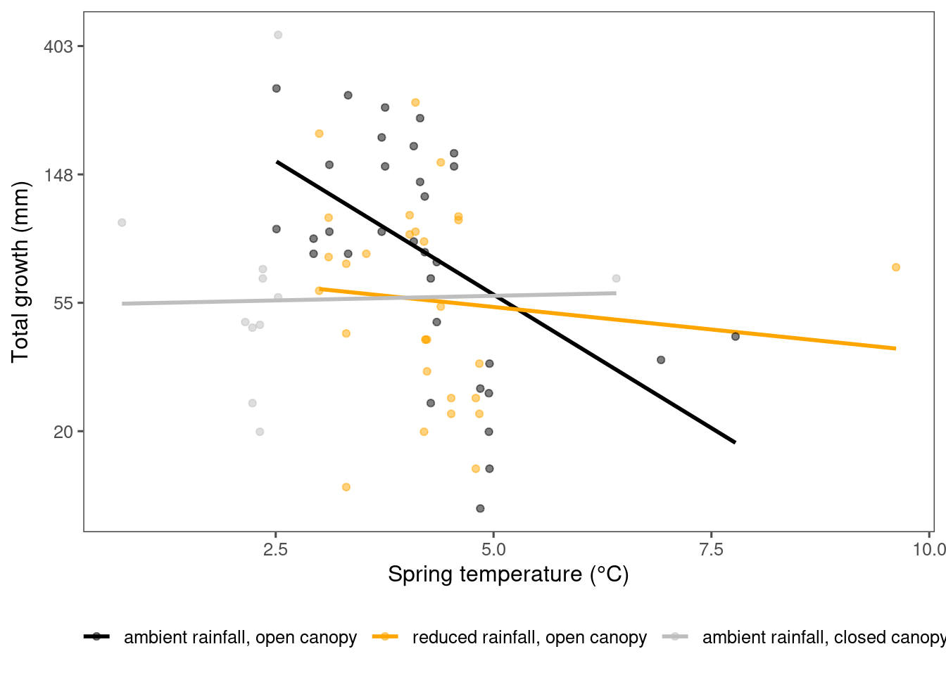

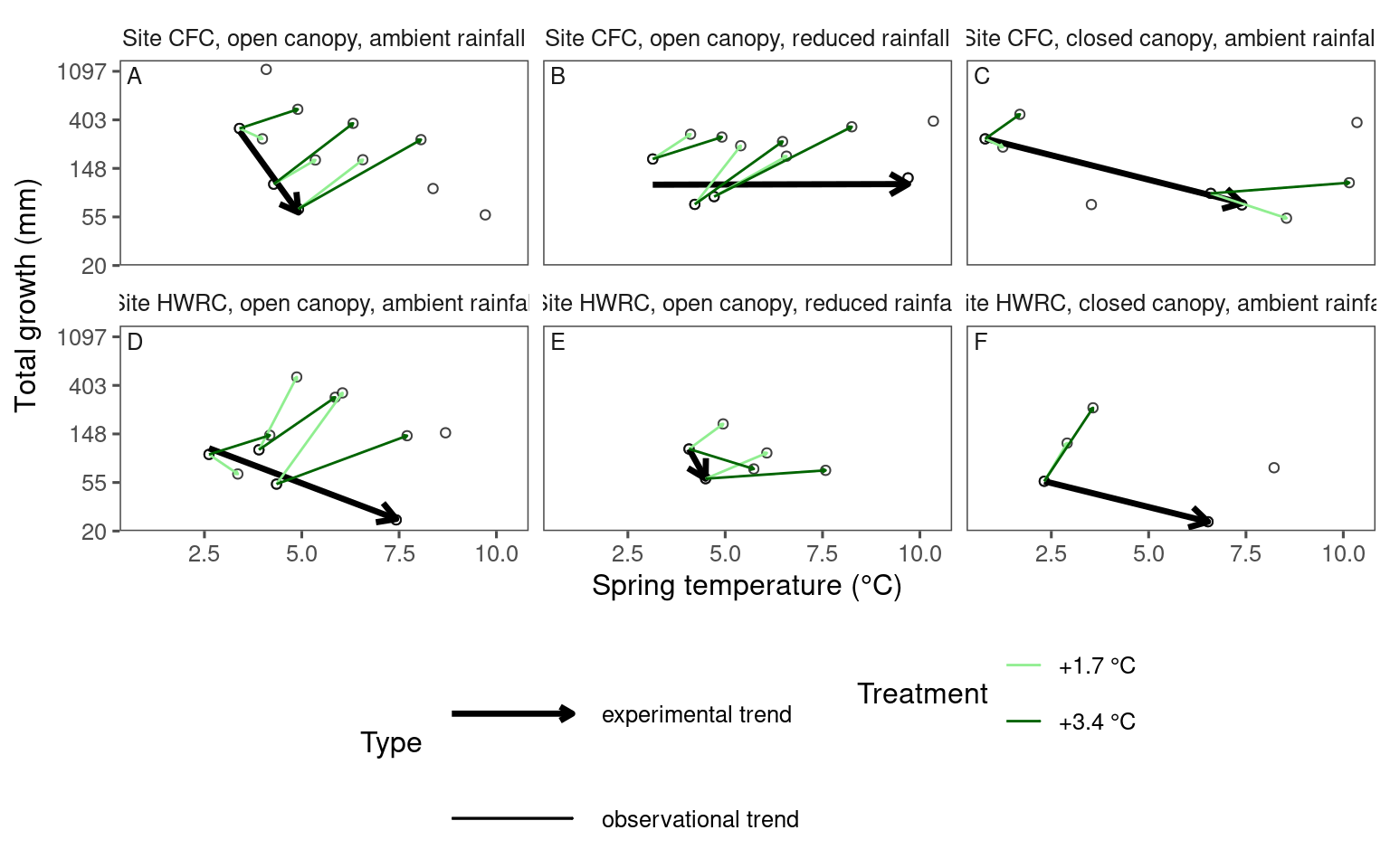
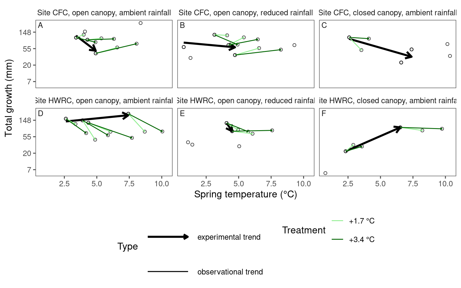
Visualizing experimental and observational trends together with arrows

dat_param_summ <- df_param_all %>%
  summ_metrics(level = "site", type = "shoot") # ignore block and plot

dat_climate_spring_summ <- summ_climate_season(dat_climate_daily, date_start = "Mar 15", date_end = "May 15", rainfall = 1, level = "site")

plot_trend(
  df = dat_param_summ %>%
    filter(param == "total growth") %>%
    filter(species == "acesa"),
  dat_climate = dat_climate_spring_summ,
  type = "shoot",
  side_by_side = F
)

plot_trend(
  df = dat_param_summ %>%
    filter(param == "total growth") %>%
    filter(species == "picgl"),
  dat_climate = dat_climate_spring_summ,
  type = "shoot",
  side_by_side = F
)

Plot comparisons of coefficients

Train model with temperature difference, baseline temperature, and the interaction of the two.

dat_climate_spring_ambient <- calc_climate_ambient(dat_climate = dat_climate_spring, dat_shoot_alive)
dat_climate_spring_diff <- calc_climate_diff(dat_climate = dat_climate_spring, dat_climate_ambient = dat_climate_spring_ambient)
(df_treatment_effect_on_climate <- summ_treatment_effect_on_climate(dat_climate_spring_diff))

## # A tibble: 9 × 5
##   heat_name water_name canopy temp             mois              
##   <fct>     <fct>      <fct>  <chr>            <chr>             
## 1 ambient   ambient    open   -0.0391 ± 0.165  0.00346 ± 0.0262  
## 2 +1.7 °C   ambient    open   1.03 ± 0.485     0.00277 ± 0.0253  
## 3 +3.4 °C   ambient    open   1.99 ± 0.815     -0.00772 ± 0.0233 
## 4 ambient   reduced    open   0.000266 ± 0.157 -0.000221 ± 0.0126
## 5 +1.7 °C   reduced    open   0.837 ± 0.677    0.00332 ± 0.0244  
## 6 +3.4 °C   reduced    open   1.76 ± 0.993     -0.00653 ± 0.0178 
## 7 ambient   ambient    closed -0.00411 ± 0.17  0.00116 ± 0.0384  
## 8 +1.7 °C   ambient    closed 1.07 ± 0.532     0.00251 ± 0.0374  
## 9 +3.4 °C   ambient    closed 2.08 ± 0.97      -0.0033 ± 0.0366

Examine number of years

dat_shoot_alive %>%
  group_by(species, canopy, water_name) %>%
  summarise(n_year = n_distinct(year)) %>%
  arrange(n_year)

## # A tibble: 45 × 4
## # Groups:   species, canopy [31]
##    species canopy water_name n_year
##    <chr>   <fct>  <fct>       <int>
##  1 fraal   open   ambient         1
##  2 fraal   open   reduced         1
##  3 lonmo   open   ambient         1
##  4 lonmo   open   reduced         1
##  5 lonta   open   ambient         1
##  6 lonta   open   reduced         1
##  7 abiba   closed ambient         4
##  8 acene   closed ambient         4
##  9 acesa   closed ambient         4
## 10 betal   closed ambient         4
## # ℹ 35 more rows

dat_shoot_all_cov <- dat_shoot_alive %>%
  tidy_shoot_extend() %>%
  filter(doy > 90, doy <= 210) %>%
  mutate(model = str_c(species, canopy, water_name, sep = "_")) %>%
  group_by(species, model) %>%
  filter(n_distinct(year) >= 4) %>%
  ungroup() %>%
  left_join(dat_climate_spring_diff) %>%
  drop_na(delta_temp_std, base_temp_std) %>%
  group_by(species, model) %>%
  mutate(group = str_c(site, year, sep = "_") %>% factor() %>% as.integer()) %>% # site-year level random effects
  ungroup() %>%
  tidy_treatment_code() %>%
  {
    # Extract only the `center` and `std` attributes
    attributes(.)$center <- attr(dat_climate_spring_diff, "center")
    attributes(.)$sd <- attr(dat_climate_spring_diff, "sd")
    .
  }

I used a model with continuous temperature difference (with ambient), continuous baseline temperature, and their interaction.

calc_bayes_all(
  data = dat_shoot_all_cov,
  independent_priors = F, # do not use species-specific empirical informative priors
  uniform_priors = T, # use uniform priors
  intui_param = F, # regular parameterization with A, x0, logk
  continuous_cov = T, # continuous treatment,
  background = T, # background temperature
  num_iterations = 50000,
  nthin = 5,
  path = "alldata/intermediate/shootmodeling/continuous_bg/",
  num_cores = 35
)
calc_bayes_derived(path = "alldata/intermediate/shootmodeling/continuous_bg/", num_cores = 35)
plot_bayes_all(path = "alldata/intermediate/shootmodeling/continuous_bg/", num_cores = 35)

I also tried a version that experimental treatment was discrete and baseline temperature was continuous.

calc_bayes_all(
  data = dat_shoot_all_cov,
  independent_priors = F, # do not use species-specific empirical informative priors
  uniform_priors = T, # use uniform priors
  intui_param = F, # regular parameterization with A, x0, logk
  continuous_cov = F, # discrete treatment,
  background = T, # background temperature
  num_iterations = 50000,
  nthin = 5,
  path = "alldata/intermediate/shootmodeling/discrete_bg/",
  num_cores = 35
)
calc_bayes_derived(path = "alldata/intermediate/shootmodeling/discrete_bg/", num_cores = 35)
plot_bayes_all(path = "alldata/intermediate/shootmodeling/discrete_bg/", num_cores = 35)

df_bayes_all <- read_bayes_all(path = "alldata/intermediate/shootmodeling/continuous_bg/", full_factorial = F, derived = T, tidy_mcmc = T) %>%
  tidy_model_name() %>%
  tidy_species_name()

p_bayes_summ <- plot_bayes_summary(
  df_bayes_all %>%
    filter(response == "total growth") %>%
    filter(covariate == "warming"),
  background = "full"
)
p_bayes_summ$p_coef_line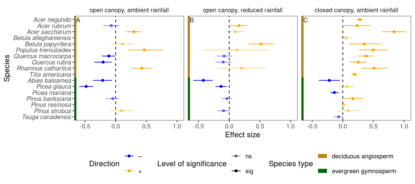

p_bayes_summ <- plot_bayes_summary(
  df_bayes_all %>%
    filter(response == "total growth") %>%
    filter(covariate == "temperature"),
  background = "full"
)
p_bayes_summ$p_coef_line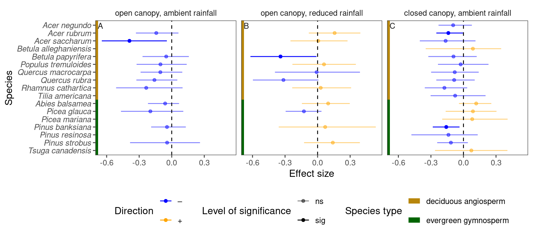

p_bayes_summ <- plot_bayes_summary(
  df_bayes_all %>%
    filter(response == "start") %>%
    filter(covariate == "warming x temperature"),
  background = "full"
)
p_bayes_summ$p_coef_line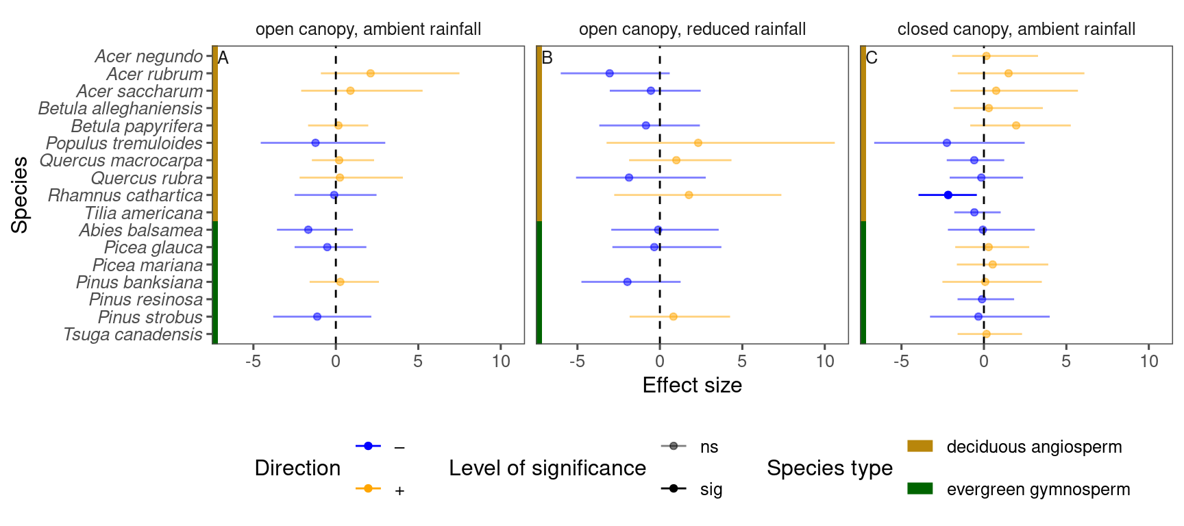

df_compare_trends <- test_compare_trends(df = df_bayes_all, v_response = c("total growth", "midpoint"))

plot_trend_compare(df_compare_trends %>% filter(response == "total growth"), type = "shoot", species_label = T, ci = F)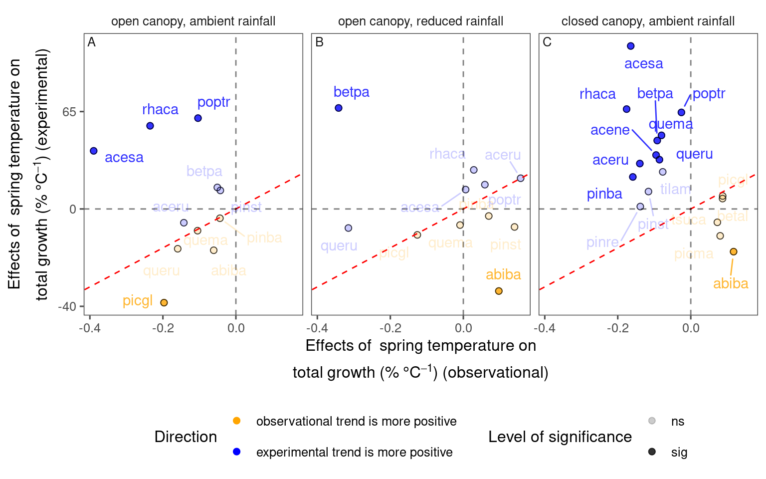

df_compare_trends %>%
  filter(response == "total growth") %>%
  group_by(sign, sig) %>%
  summarise(n = n(), .groups = "drop") %>%
  mutate(perc = n / sum(n))

## # A tibble: 4 × 4
##   sign  sig       n   perc
##   <chr> <chr> <int>  <dbl>
## 1 +     ns       11 0.282 
## 2 +     sig      13 0.333 
## 3 –     ns       12 0.308 
## 4 –     sig       3 0.0769