Pre-process data
This time I use the data slightly updated in the previous blog.
dat_shoot %>%
  drop_na(barcode) %>%
  filter(shoot > 0) %>%
  filter(!is.na(shoot)) %>%
  group_by(barcode, year) %>%
  summarize(alive = if_else(any(alive == 0), 0, 1), .groups = "drop") %>%
  group_by(alive) %>%
  summarize(n = n()) %>%
  mutate(perc = n / sum(n))
## # A tibble: 2 × 3
## alive n perc
## <dbl> <int> <dbl>
## 1 0 389 0.0682
## 2 1 5316 0.932dat_shoot %>%
drop_na(barcode) %>%
filter(shoot > 0) %>%
filter(!is.na(shoot)) %>%
group_by(species, water_name, canopy, barcode, year) %>%
summarize(alive = if_else(any(alive == 0), 0, 1), .groups = "drop") %>%
group_by(species, water_name, canopy) %>%
summarize(alive_perc = sum(alive) / n() * 100, .groups = "drop") %>%
arrange(alive_perc) %>%
head(15)## # A tibble: 15 × 4
## species water_name canopy alive_perc
## <chr> <fct> <fct> <dbl>
## 1 poptr ambient closed 67.5
## 2 betpa ambient closed 70
## 3 poptr ambient open 79.5
## 4 aceru ambient closed 81.6
## 5 pinba ambient closed 82.6
## 6 queru ambient closed 82.6
## 7 rhaca ambient closed 85
## 8 acesa ambient closed 86.2
## 9 poptr reduced open 86.8
## 10 quema ambient closed 87.5
## 11 pinst ambient closed 87.8
## 12 betpa reduced open 88.0
## 13 betpa ambient open 89.8
## 14 rhaca ambient open 90.2
## 15 picgl reduced open 90.4This time, I choose to filter out plants that have been determined to be dead at any point in a year.
dat_shoot_alive <- dat_shoot %>%
  drop_na(barcode) %>%
  filter(shoot > 0) %>%
  filter(!is.na(shoot)) %>%
  group_by(barcode, year) %>%
  mutate(shoot_alive = if_else(any(alive == 0), 0, 1)) %>% # filter out plants ever considered dead at any point in a year
  ungroup() %>%
  filter(shoot_alive == 1) %>%
  select(-alive, -shoot_alive) %>%
  tidy_shoot_extend()

# dat_shoot_dead <- dat_shoot %>%
#   filter(shoot > 0) %>%
#   filter(!is.na(shoot)) %>%
#   group_by(barcode, year) %>%
#   mutate(shoot_alive = if_else(any(alive == 0), 0, 1)) %>%
#   ungroup() %>%
#   filter(shoot_alive == 0)

dat_all <- dat_shoot_alive %>%
  filter(doy > 90, doy <= 210) %>%
  mutate(model = str_c(species, canopy, water_name, sep = "_")) %>%
  group_by(species, model) %>%
  mutate(group = str_c(site, year, sep = "_") %>% factor() %>% as.integer()) %>% # site-year level random effects
  ungroup() %>%
  tidy_treatment_code()
Shoot growth model
Data model
\[\begin{align*} y_{i,t,s,d} \sim \text{Lognormal}(\mu_{i,t,s,d}, \sigma^2) \end{align*}\]
Process model
\[\begin{align*} \mu_{i,t,s,d} &= c+\frac{A_{i,t,s}}{1+e^{-k_{i,t,s}(d-x_{0 i,t,s})}} \newline A_{i,t,s} &= \mu_A + \delta_{A,i}+ \alpha_{A,t,s} \newline x_{0 i,t,s} &= \mu_{x_0} + \delta_{x_0,i}+ \alpha_{x_0,t,s} \newline log(k_{i,t,s}) &= \mu_{log(k)} + \delta_{log(k),i}+ \alpha_{log(k),t,s} \end{align*}\]
Fixed effects
\[\begin{align*} \delta_{A,i} &= \beta_{A,1} W_i \newline \delta_{x_0,i} &= \beta_{x_0,1} W_i \newline \delta_{log(k),i} &= \beta_{log(k),1} W_i \end{align*}\]
Random effects
\[\begin{align*} \alpha_{A,t,s} &\sim \text{Normal}(0, \sigma_A^2) \newline \alpha_{x_0,t,s} &\sim \text{Normal}(0, \sigma_{x_0}^2) \newline \alpha_{log(k),t,s} &\sim \text{Normal}(0, \sigma_{log(k)}^2) \end{align*}\]
Priors
\[\begin{align*} c &\sim \text{Uniform}(0, 1) \newline \mu_A &\sim \text{Uniform}(1, 6) \newline \beta_A &\sim \text{Normal} (0,0.5)\newline \sigma_A &\sim \text{Truncated Normal}(0, 0.5, 0, \infty) \newline \mu_{x_0} &\sim \text{Uniform}(120, 180) \newline \beta_{x_0} &\sim \text{Normal} (0,5)\newline \sigma_{x_0} &\sim \text{Truncated Normal}(0, 5, 0, \infty) \newline \mu_{log(k)} &\sim \text{Uniform}(-3.5, -1) \newline \beta_{log(k)} &\sim \text{Normal} (0,0.1)\newline \sigma_{log(k)}^2 &\sim \text{Truncated Normal}(0, 0.1, 0, \infty) \newline \sigma^2 &\sim \text{Truncated Normal}(0, 1, 0, \infty) \end{align*}\]
This time, I tightened the priors a bit because of poptr and betpa had large variability but lacked data after using separate models. I had to impose stronger regularization to reduce the risk of overfitting.
Fit model
calc_bayes_all(
  data = dat_all,
  independent_priors = F, # do not use species-specific empirical informative priors
  uniform_priors = T, # use uniform priors
  intui_param = F, # regular parameterization with asym, xmid, logk
  num_iterations = 50000,
  nthin = 5,
  path = "alldata/intermediate/shootmodeling/separate_models/",
  num_cores = 35
)
calc_bayes_derived(path = "alldata/intermediate/shootmodeling/separate_models/", num_cores = 35)
plot_bayes_all(path = "alldata/intermediate/shootmodeling/separate_models/", num_cores = 35)
MCMC
df_bayes_all <- read_bayes_all(path = "alldata/intermediate/shootmodeling/separate_models/", full_factorial = F, derived = F, tidy_mcmc = F)p_bayes_diagnostics <- plot_bayes_diagnostics(df_MCMC = df_bayes_all %>% filter(model == "aceru_open_ambient"), plot_corr = F)
p_bayes_diagnostics$p_MCMC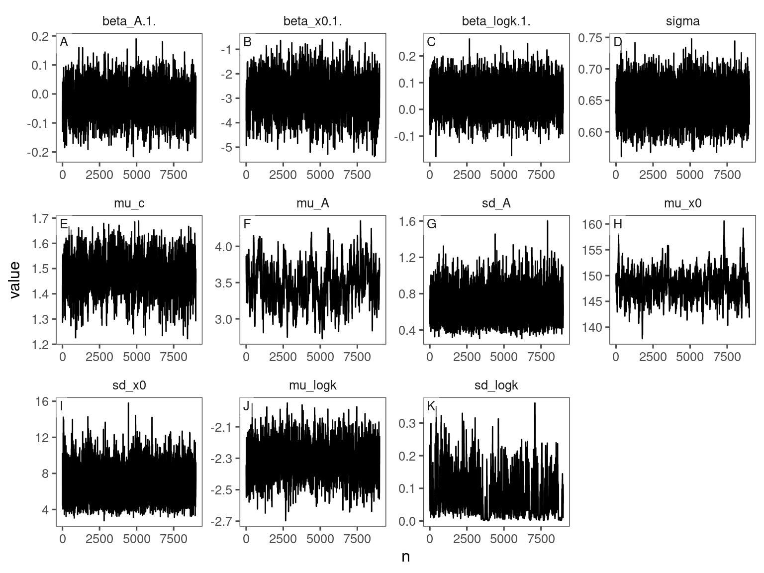
p_bayes_diagnostics$p_posterior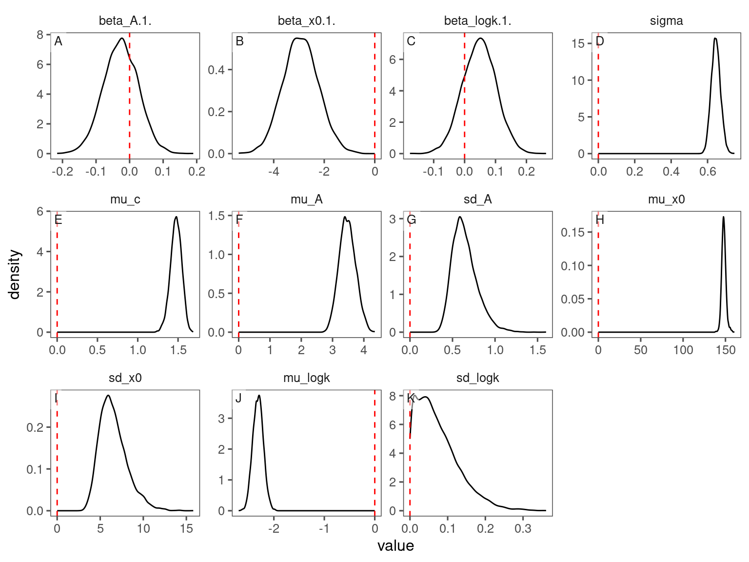
Conditional predictions
df_bayes_pred_all <- read_bayes_all(path = "alldata/intermediate/shootmodeling/separate_models/", full_factorial = F, content = "predict")

p_bayes_predict <- plot_bayes_predict(
  data = dat_all %>% filter(species == "aceru"),
  data_predict = df_bayes_pred_all %>% filter(str_detect(model, "aceru")),
  vis_log = T,
  vis_ci = F
)

p_bayes_predict$p_overlay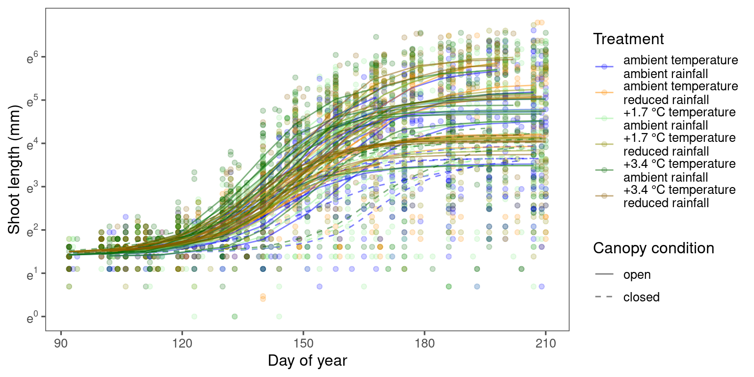
Accuracy
p_bayes_predict$p_accuracy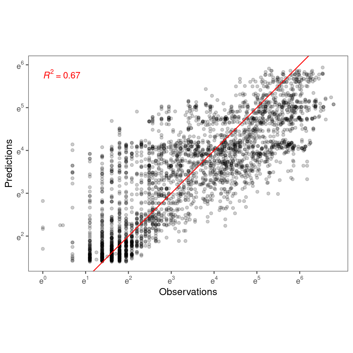
Marginal predictions
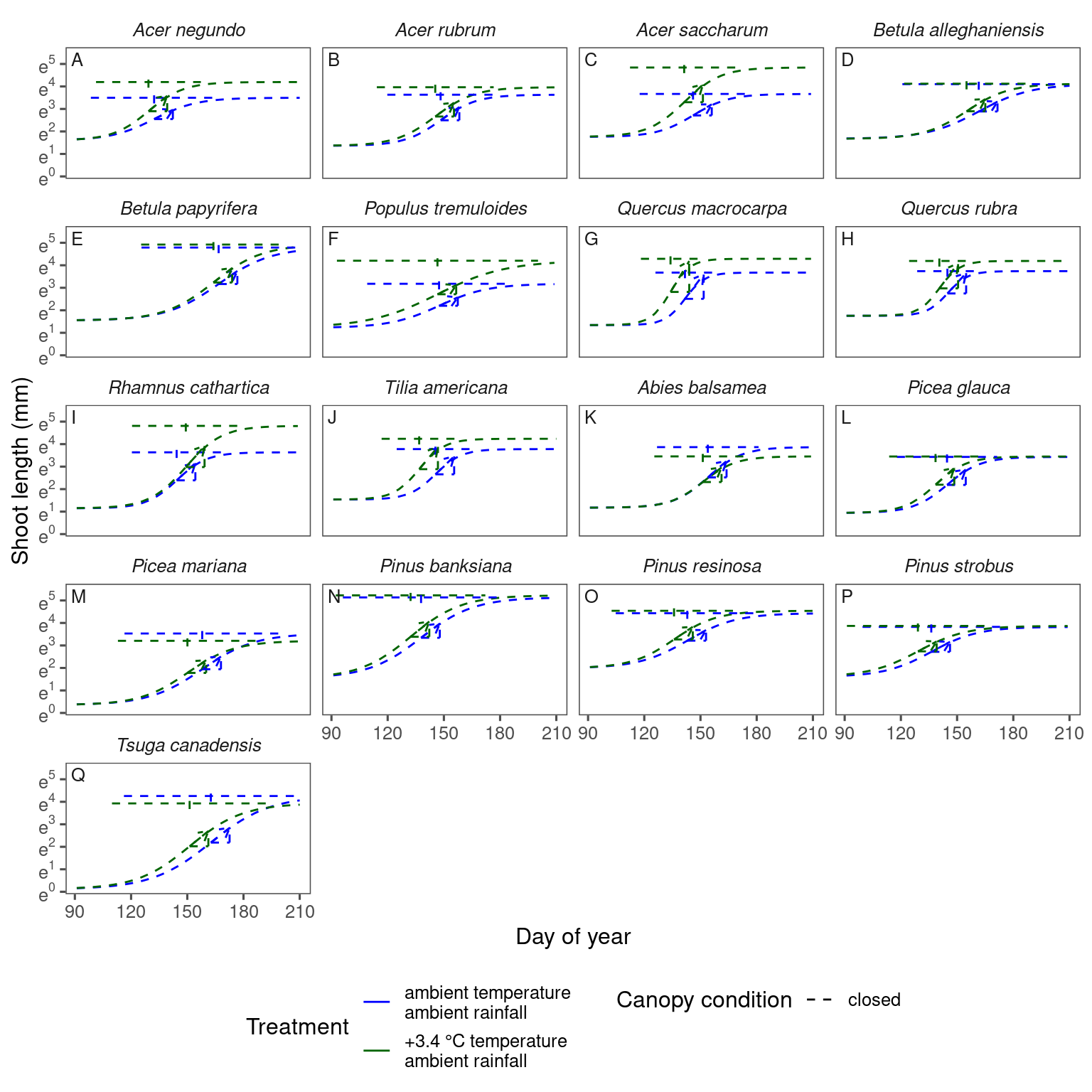
df_bayes_pred_marginal_all <- read_bayes_all(path = "alldata/intermediate/shootmodeling/separate_models/", full_factorial = F, content = "predict_marginal")

p_bayes_predict <- plot_bayes_predict(
  data_predict = df_bayes_pred_marginal_all %>% filter(str_detect(model, "aceru")),
  vis_log = T,
  vis_ci = F
)
p_bayes_predict$p_predict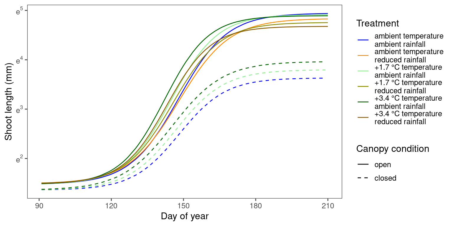
Coefficients
Read in summary of inferred parameters
df_bayes_all <- read_bayes_all(path = "alldata/intermediate/shootmodeling/separate_models/", full_factorial = F, derived = T, tidy_mcmc = T) %>%
  tidy_species_name() %>%
  tidy_model_name() %>%
  mutate(value = value * (str_detect(param, "beta") + 1)) # effect of 3.4 degree C warming instead of 1.7 degree C
Intercept
p_bayes_summ <- plot_bayes_summary(df_bayes_all, option = "mu", derived_metric = "asymptote_focused")
p_bayes_summ$p_coef_line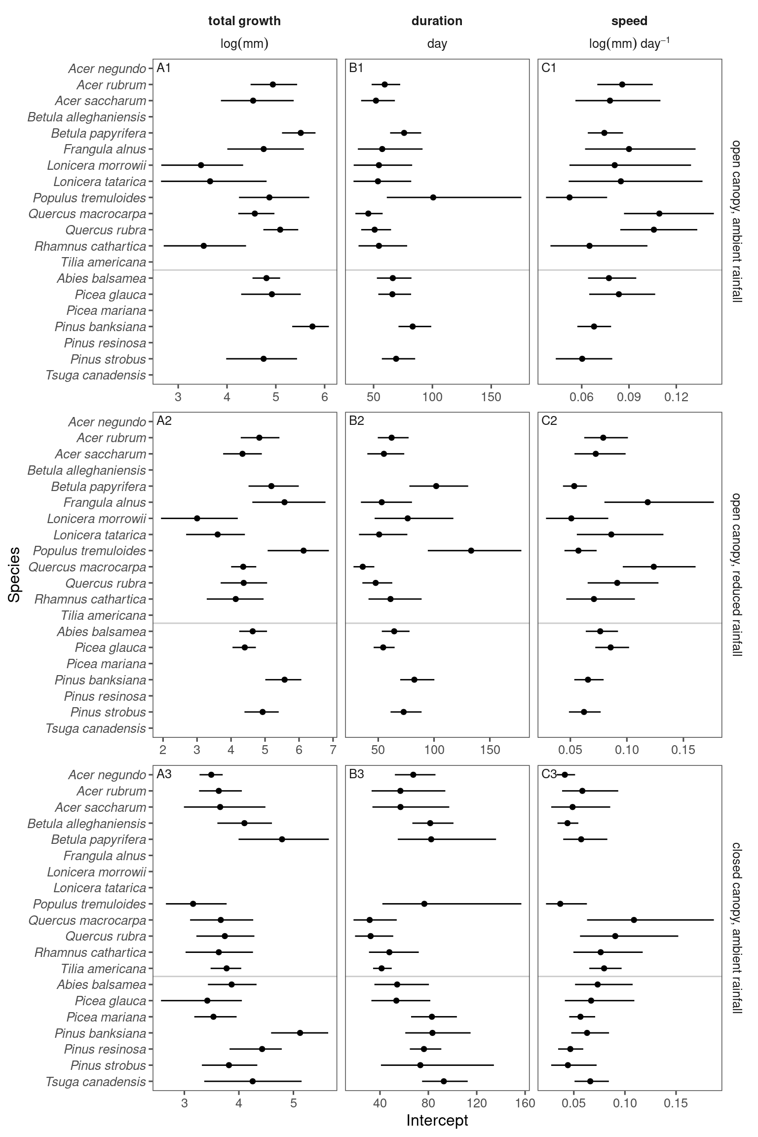
p_bayes_summ <- plot_bayes_summary(df_bayes_all, option = "mu", derived_metric = "no")
p_bayes_summ$p_coef_line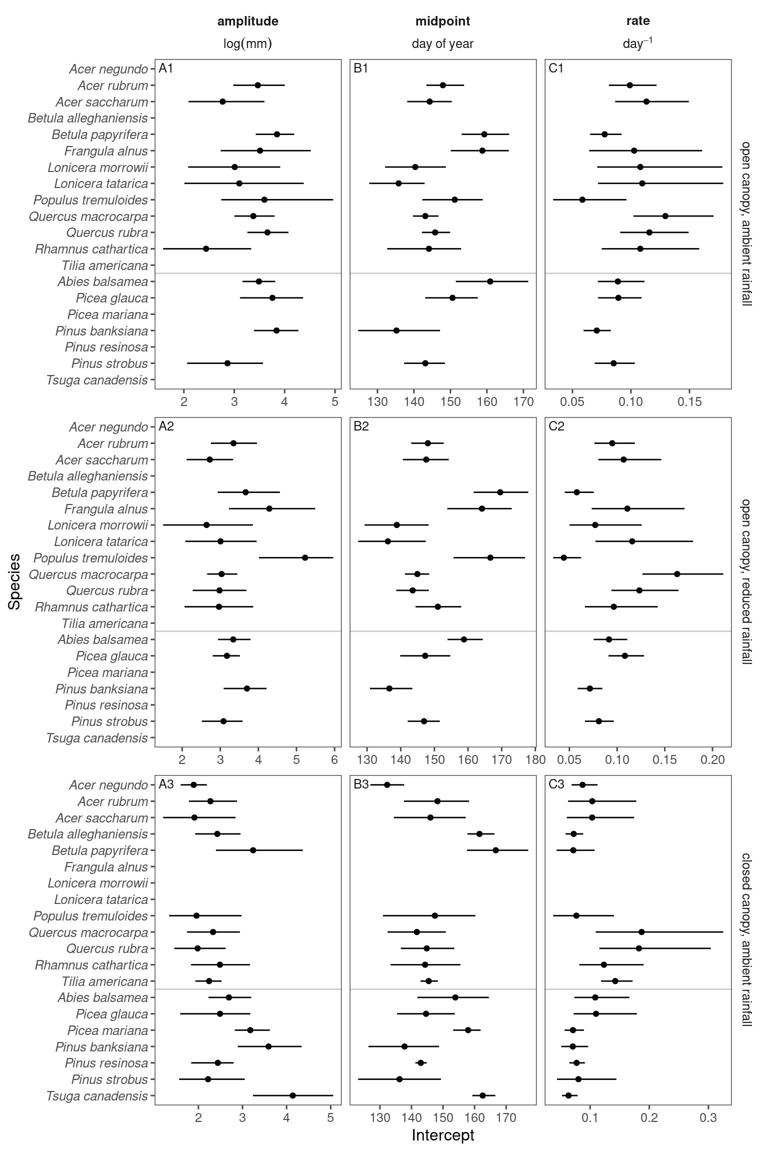
Coefficients
p_bayes_summ <- plot_bayes_summary(df_bayes_all, option = "coef", derived_metric = "asymptote_focused")
p_bayes_summ$p_coef_line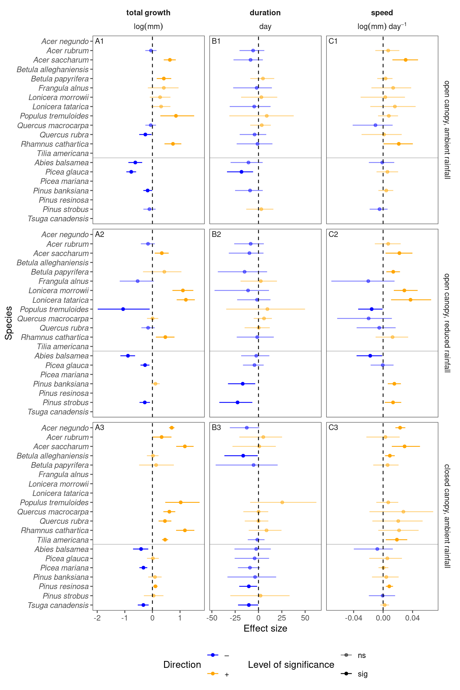
p_bayes_summ <- plot_bayes_summary(df_bayes_all, option = "coef", derived_metric = "no")
p_bayes_summ$p_coef_line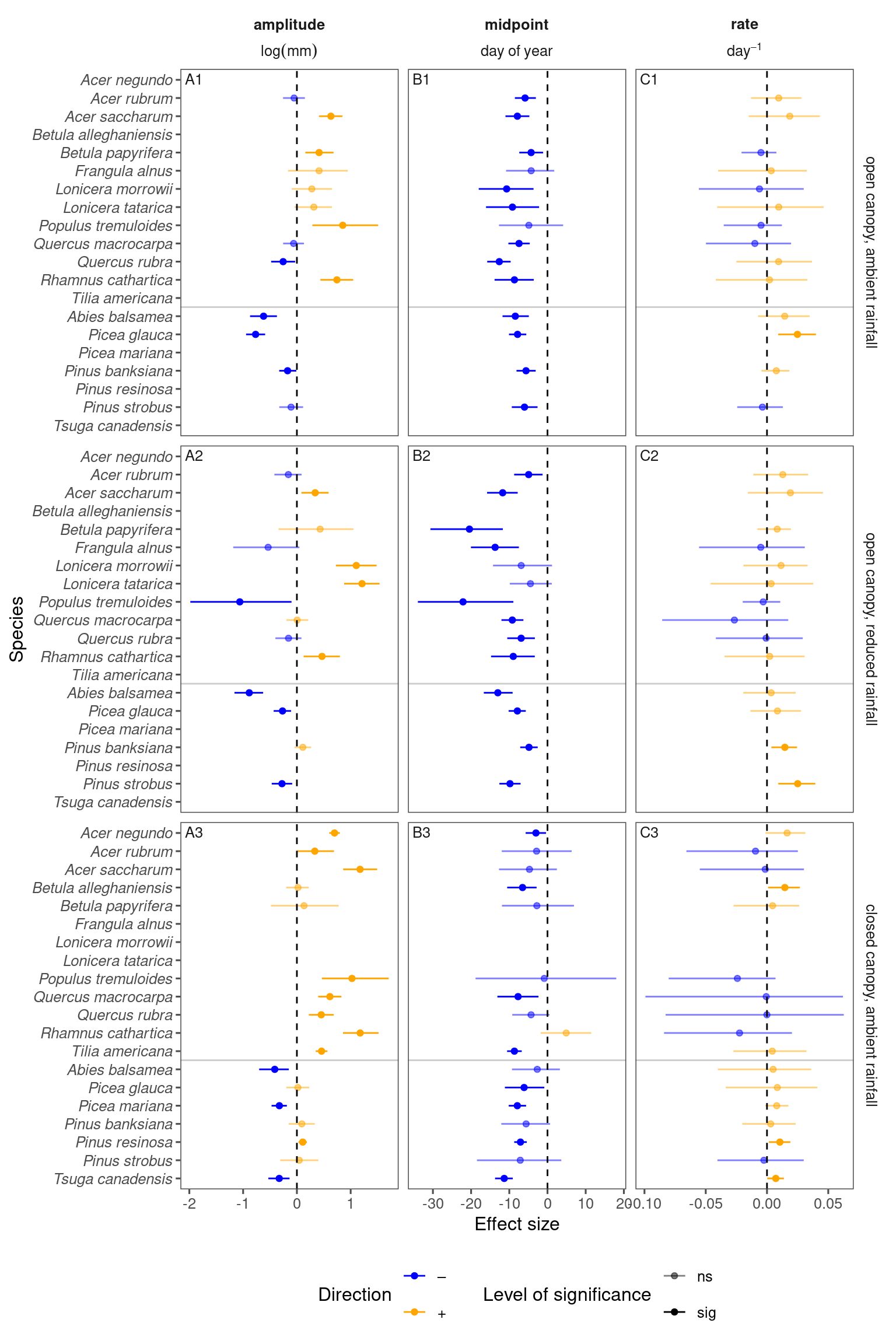
Composite figure
p_bayes_summ <- plot_bayes_summary(df_bayes_all %>% filter(response == "midpoint"), option = "coef", derived_metric = "all")
p1 <- p_bayes_summ$p_coef_line +
  xlab("Effect size on midpoint    day")
p_bayes_summ <- plot_bayes_summary(df_bayes_all %>% filter(response == "total growth"), option = "coef", derived_metric = "all")
p2 <- p_bayes_summ$p_coef_line +
xlab("Effect size on total growth log(mm)") +
tagger::tag_facets(tag_suffix = "", tag_pool = c("D", "E", "F"))df_shoot_coef <- read_bayes_all(path = "alldata/intermediate/shootmodeling/separate_models/", full_factorial = F, derived = T, tidy_mcmc = T, content = "mcmc") %>%
summ_mcmc(option = "all", stats = "median") %>%
tidy_species_name() %>%
tidy_model_name()
df_shoot_pred <- read_bayes_all(path = "alldata/intermediate/shootmodeling/separate_models/", full_factorial = F, derived = F, content = "predict_marginal") %>%
tidy_species_name() %>%
tidy_model_name()
p3 <- plot_synthesis(df_shoot_pred %>% filter(species %in% c("acesa", "picgl")),
df_shoot_coef %>% filter(species %in% c("acesa", "picgl")),
treatment = "warming", separate_models = T
) +
tagger::tag_facets(tag_suffix = "", tag_pool = c("G", "H"))wrap_elements(p1 / p2 + plot_layout(guides = "collect") & theme(legend.position = "bottom")) / wrap_elements(p3) + plot_layout(heights = c(2, 1))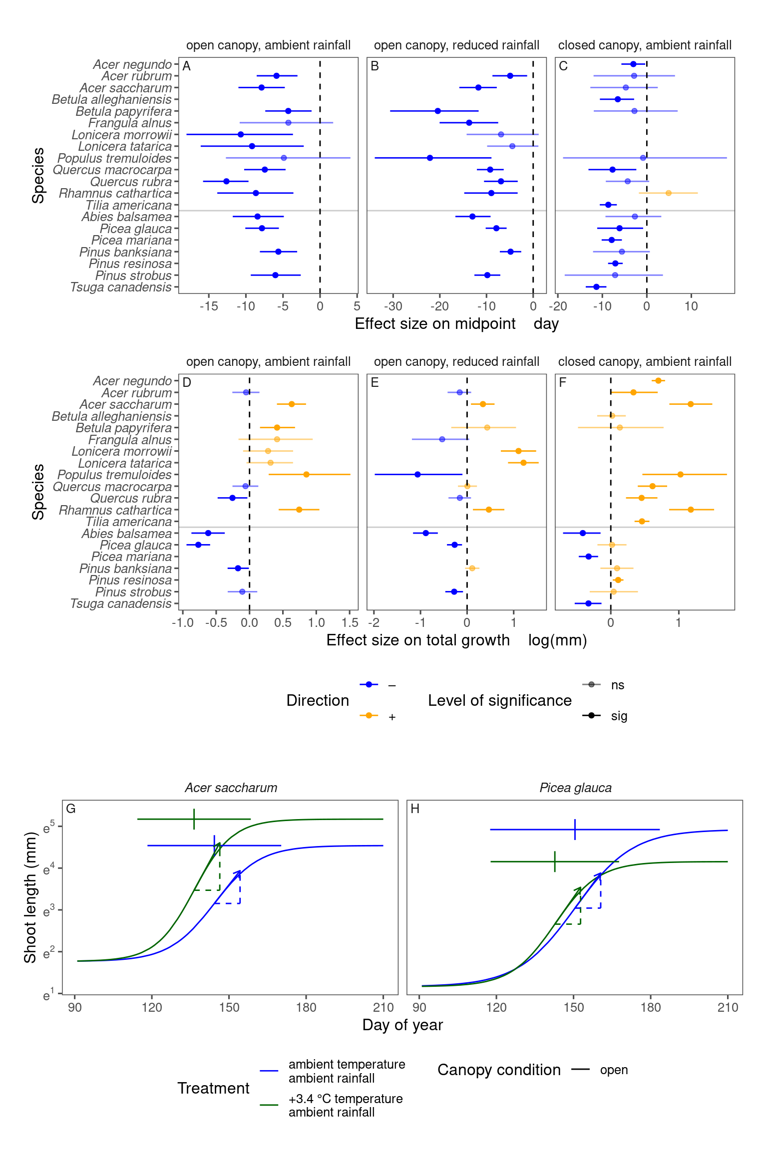
plot_synthesis(df_shoot_pred, df_shoot_coef, treatment = "warming", separate_models = T)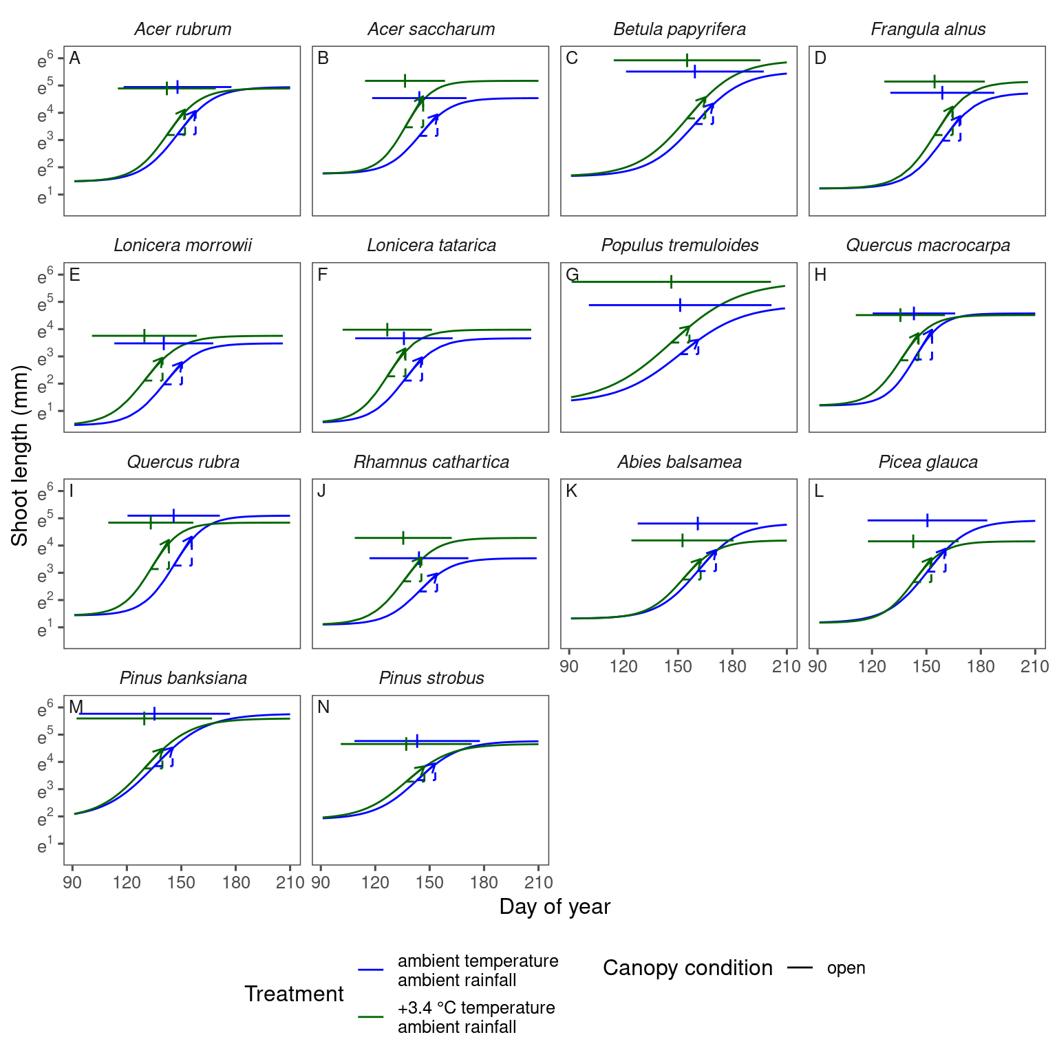
plot_synthesis(df_shoot_pred, df_shoot_coef, treatment = "warming | drying", separate_models = T)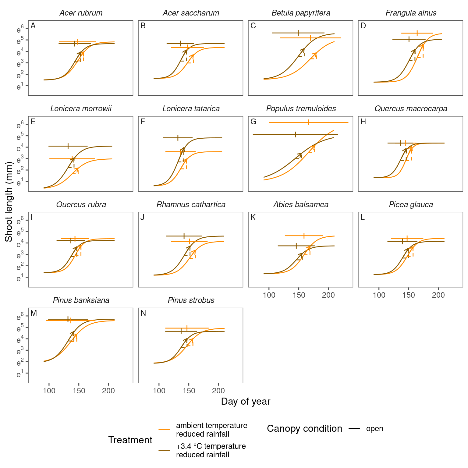
plot_synthesis(df_shoot_pred, df_shoot_coef, treatment = "warming | closed", separate_models = T)