Extract parameters

Here we no longer assume logistic growth curves.

For each growth curve for an individual shoot in a spring, we perform the following steps.

1. Log-transform shoot length.
2. Extract empirically the minimum and maximum of log(shoot length).
3. Calculate asymptote as the difference between minimum and maximum.
4. Calculate start and end of growth as the time first exceeding 5% and 95% asymptote.
5. Calculate duration as the difference between start and end.
6. Calculate speed as the maximum speed at intervals of measurements.

dat_shoot_extend <- dat_shoot %>% tidy_shoot_extend()

dat_all <- dat_shoot_extend %>%
  filter(shoot > 0) %>%
  drop_na(barcode) %>%
  select(-doy, -shoot, doy, shoot)

df_param_all <- calc_empirical_parameters(df = dat_all, path = "alldata/intermediate/", log = T)
df_param_diff <- calc_parameter_diff(df_param_all) %>%
  tidy_species_name()

Compare asymptote

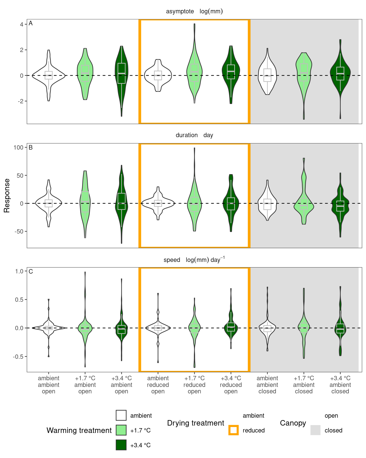
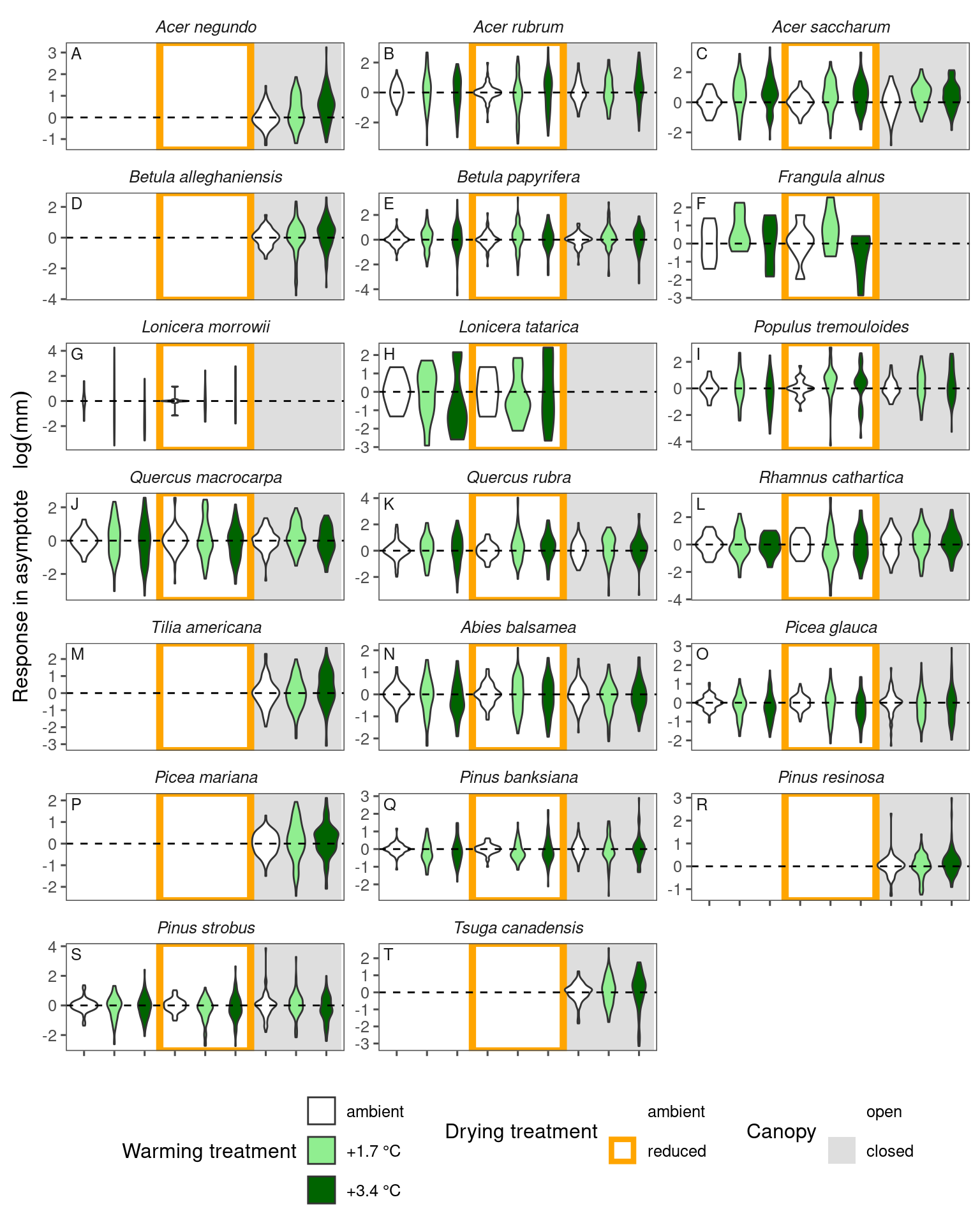
We can see an increase in asymptote for some species, e.g., acene, acesa, and decrease for some other species, e.g., pinba, pinst. These changes are qualitatively consistent with what we inferred from models, but there are several reasons that responses might differ.

1. The extraction of parameters based on noisy measurements introduced large uncertainty.
2. Here we extract parameters for individual shoots, while we pool data from individuals in the modeling approaches.
3. Here we do not take site-year-level variations into account, so any spatiotemporal bias in the presence of species might confound the results.
4. When we use a modeling approach, we assume that growth curves in the ambient and treatment groups share the same minimum values, which I think is a very fare assumption. Here because each growth curve is handled separately, there is no shared information in the minimum values. However, the asymptote is very sensitive to the minimum values.

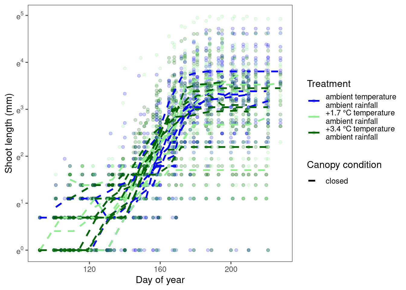
Some species, e.g., picma, showed an inconsistent trend, with asymptote increasing under warming here but decreasing in the modeling approach. What went wrong? If we plot the raw data with no model fitted, we see that the growth curves in warming treatments have lower minimum values. As a result, they have a higher asymptotes. This aligns with the #4 reason above for why we might expect different responses. This reveals a disadvantage of the empirical extraction approach.

What if we do not take log?

df_param_all_nolog <- calc_empirical_parameters(df = dat_all, path = "alldata/intermediate/", log = F)
df_param_diff_nolog <- calc_parameter_diff(df_param_all_nolog) %>%
  tidy_species_name()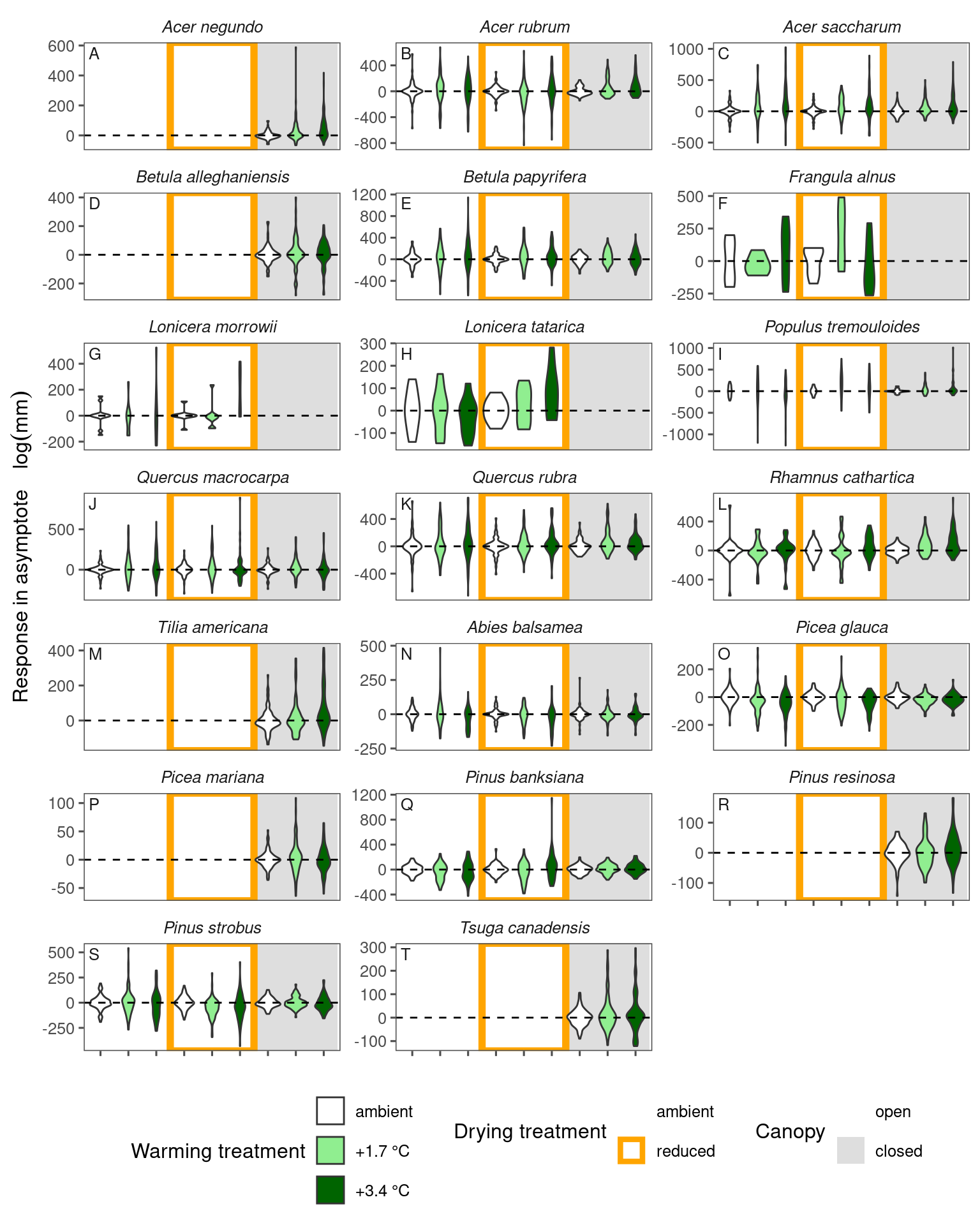

Responses are qualitatively consistent but even harder to visualize because of the large uncertainty.

Correlation between duration and speed

Previously from the Bayesian inference, we got negative correlations between duration and speed, as well as between the response in duration and response in speed.

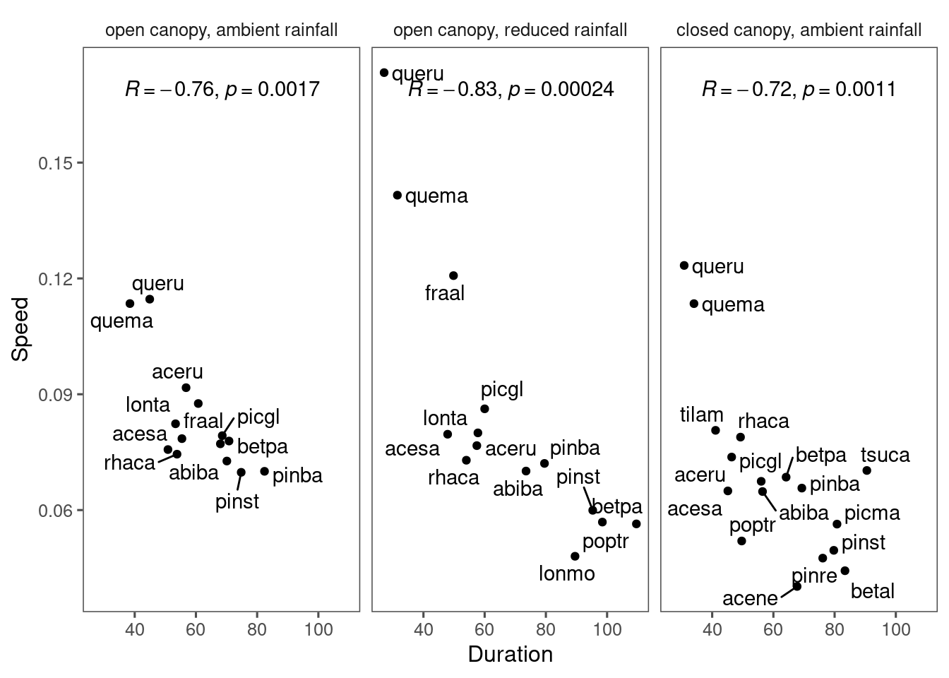
This relationship above is likely to be spurious because of the built-in correlation through parameter \(k\).

Now, we test this relationship using empirically extracted parameters.

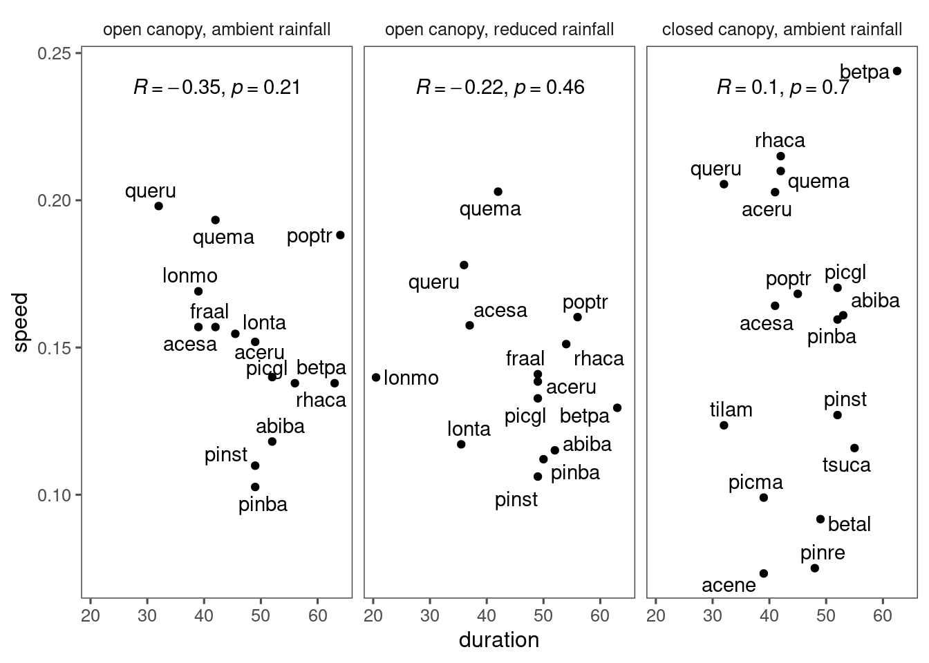No such negative correlation among species.

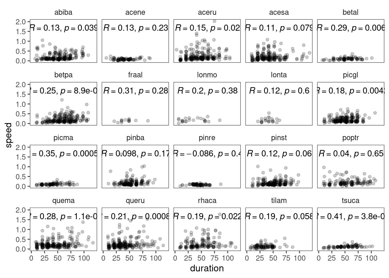
Within species, there might even be a positive relationship between duration and speed for some species.

This motivates us to reparameterize the logistic function with duration and speed, if we are interested in the relationship between these two. Will this reparameterization solve the problem entirely?