Queru in ambient rainfall vs reduced rainfall

In a previous plot, we saw unexpectedly high growth speed of red oaks in ambient temperature & reducted rainfall, compared to ambient temperature & ambient rainfall. Now we revisit the raw data to see if this is real. 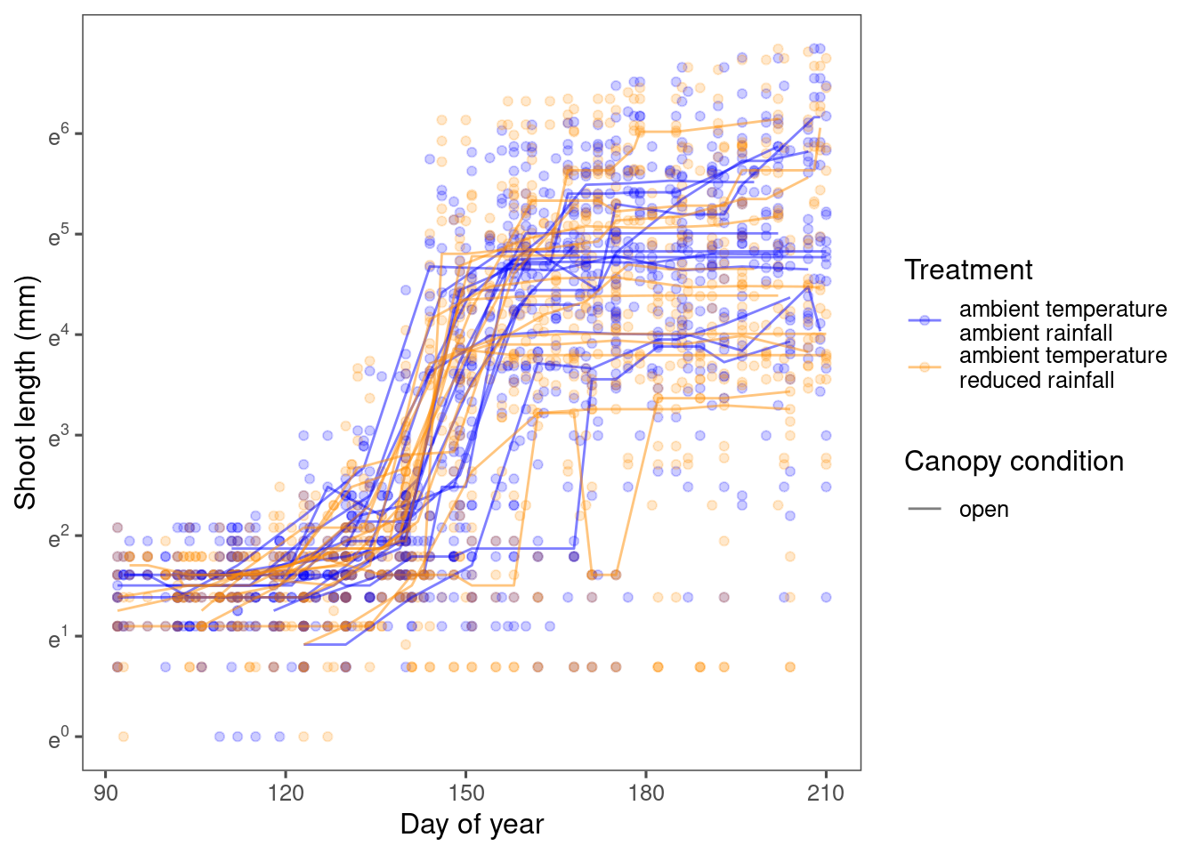The figure above has no model fitted. The lines were only from connecting the medians of observed shoot length.

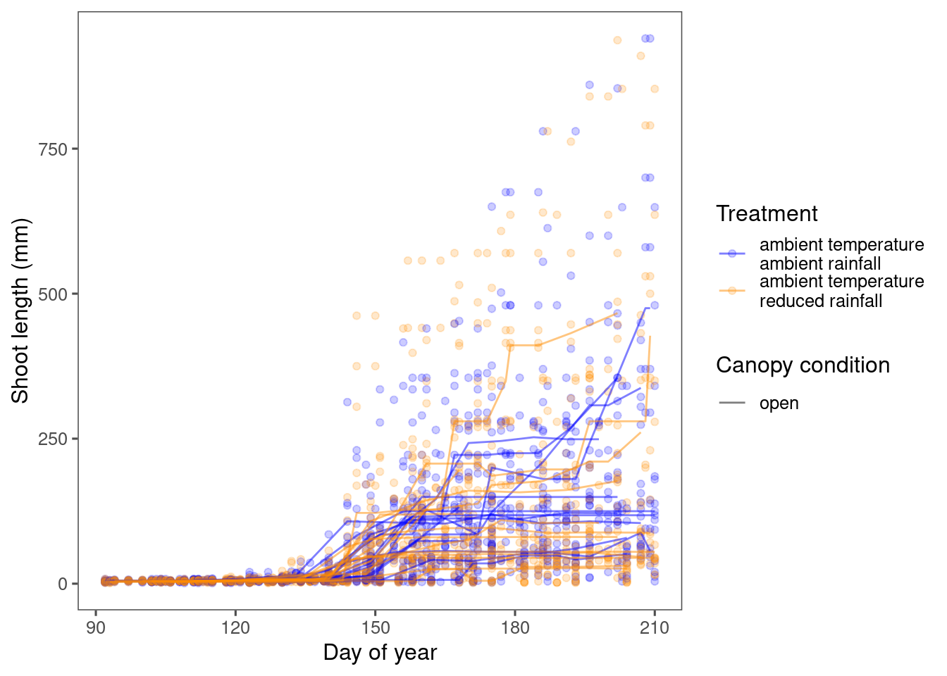
Now we apply a simple nonlinear regression model fitting.

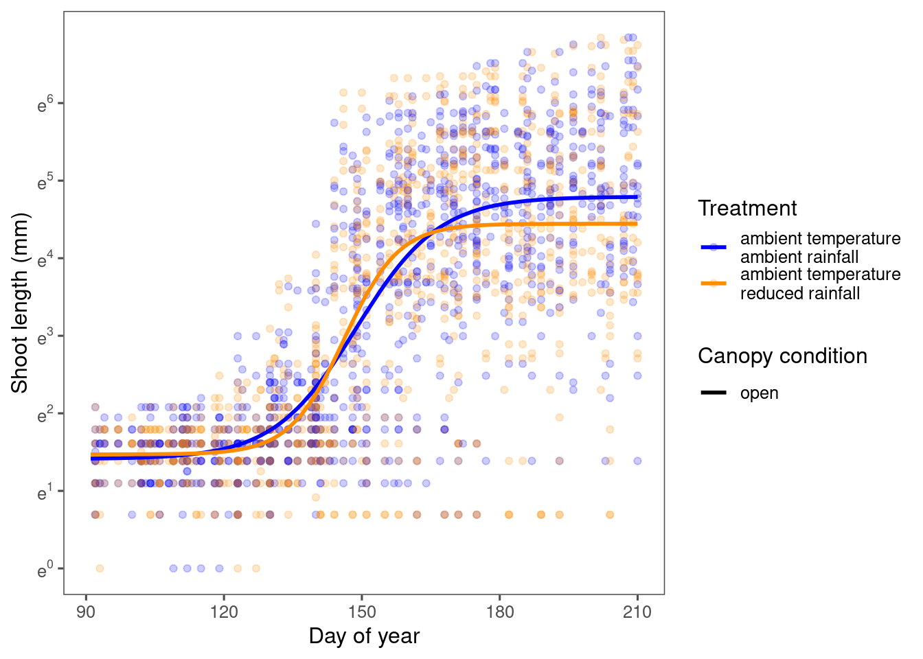
There did seem to be higher speed in reduced rainfall, but possibly from a shorter duration. Also note that the difference in speed were not significant, because of the large variations in the speed in reduced rainfall treatments.

If we visualize the non-transformed curves, the difference is still there but less visible.

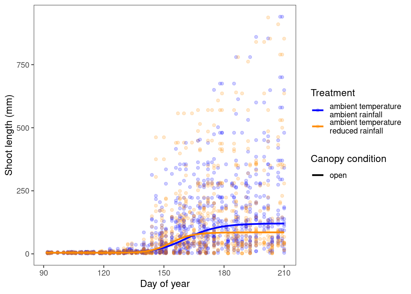
Note that this unexpected high rate of growth in reduced rainfall was not observed when using the full model, which might have stabilized the parameters.

Different species in ambient conditions

In a previous figure, I showed that evergreen species (e.g., tsuca) had higher asymptotes than deciduous species in the ambient temperature. This is counterintuitive, as we did not observe more growth in evergreen species in the field. I realized that this is likely because we assumed a logistic function for log(shoot length), such that the inferred asymptotes represent ratios instead of absolute changes. This makes the asymptote very sensitive to the starting value, which is pretty much the length of the bud over the winter.

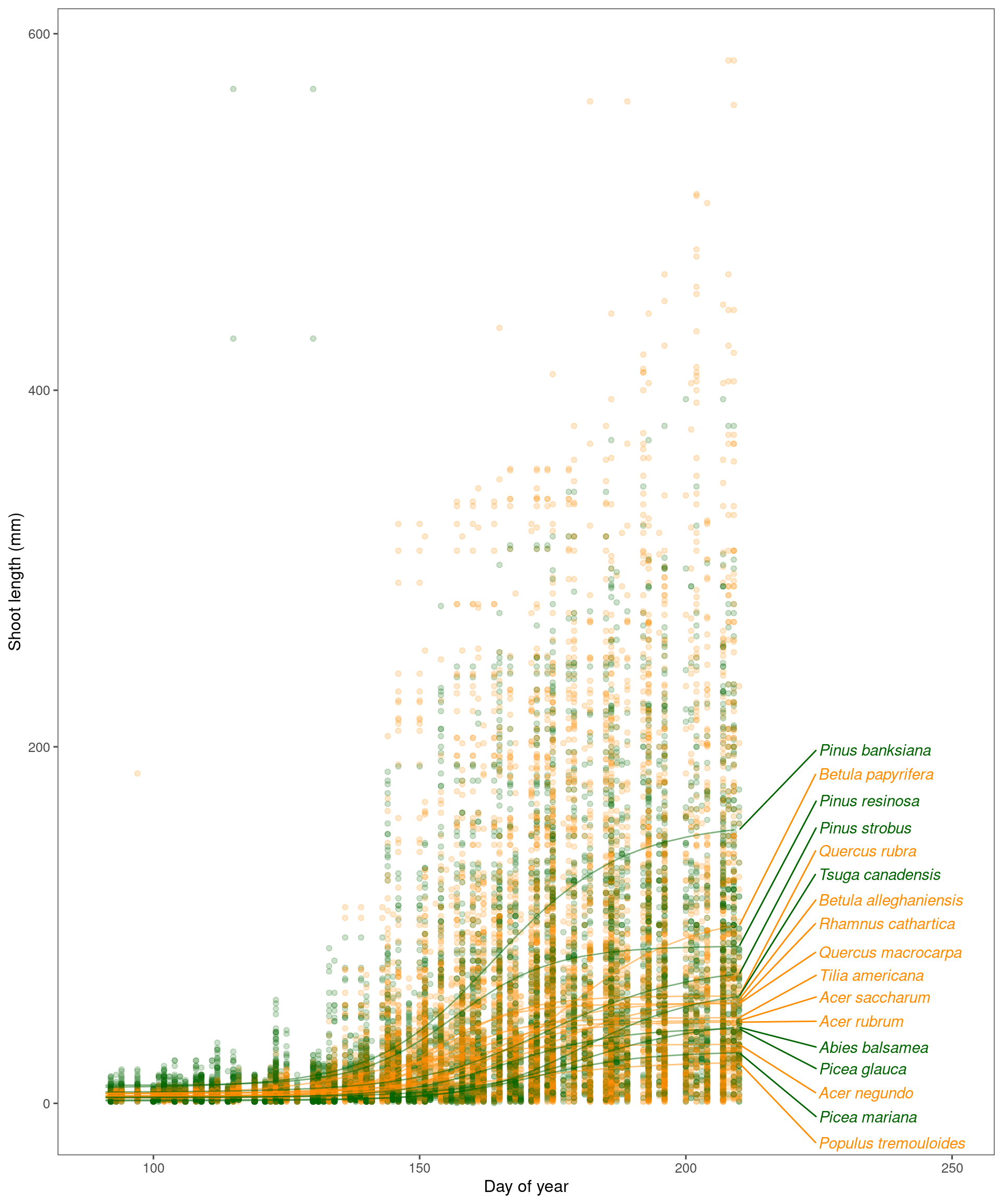
Now we compare the raw data across species in the ambient temperature, ambient rainfall, closed canopy.

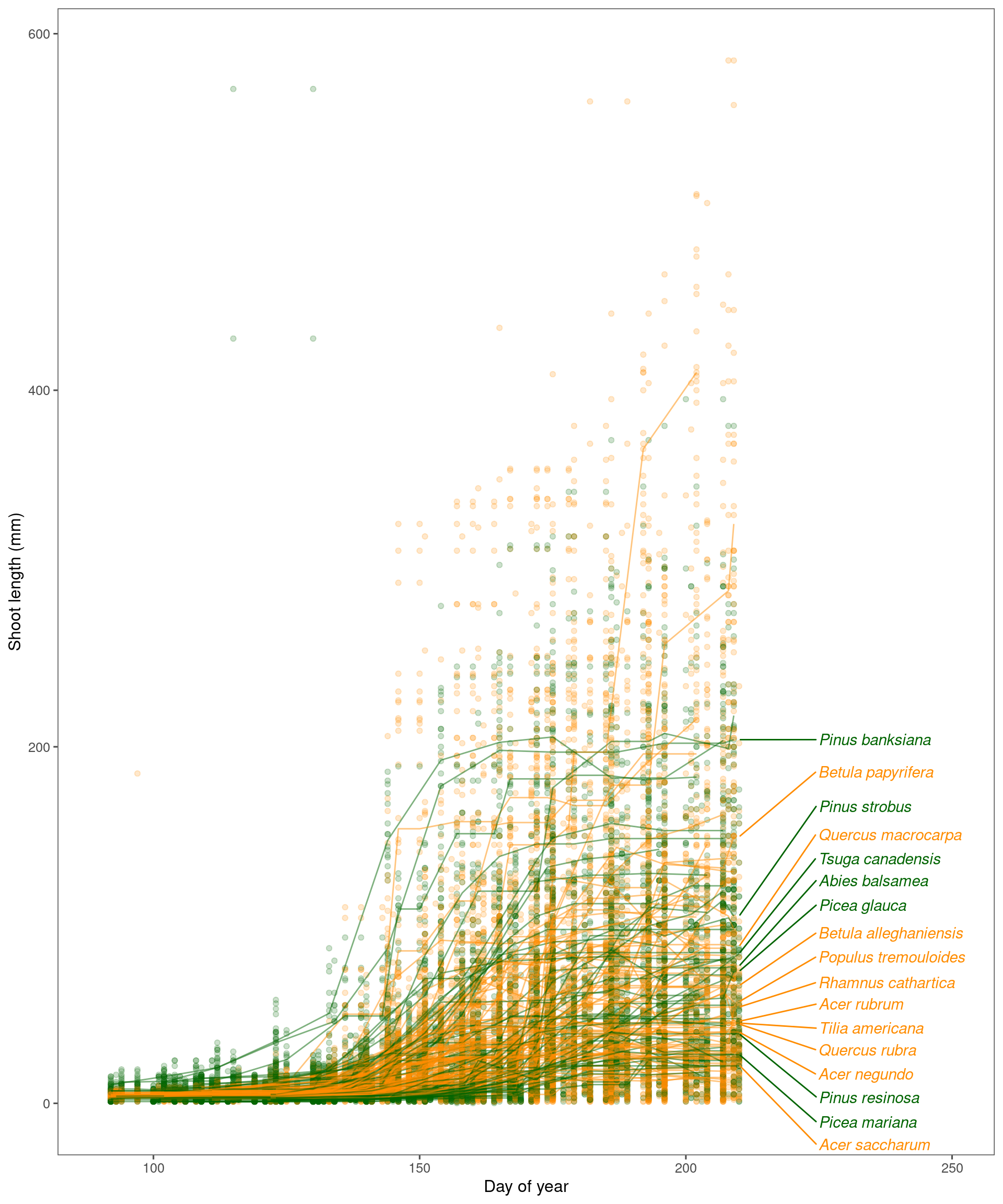No sign that evergreen species end up growing more in terms of shoot length (mm), suggesting that the previously observed pattern was mostly due to the size of buds.

Now we again plot the fitted lines from nonlinear regression.

Issues with log transformation

From the previous example, we see that the interpretation of asymptote on log scale can be easily misleading. This issue does not change our qualitative findings of positive and negative responses, but does affect the baselines and effect sizes.

For more intuitive interpretation, I can derive asymptote-related parameters back on original scale, i.e., asymptote in the unit of mm and response in asymptote also in the unit of mm.

However, how we handle midpoint, duration, and speed is much trickier.

Here I use a simulation to show that the midpoint shown in the vertial line for the log-transformed curve is not the midpoint of the original curve. The maximum speed do not occur at the same time. In addition, the 5% and 95% of increase in log(shoot length) in horizontal lines do not correspond to the 5% and 95% of increase in shoot length.

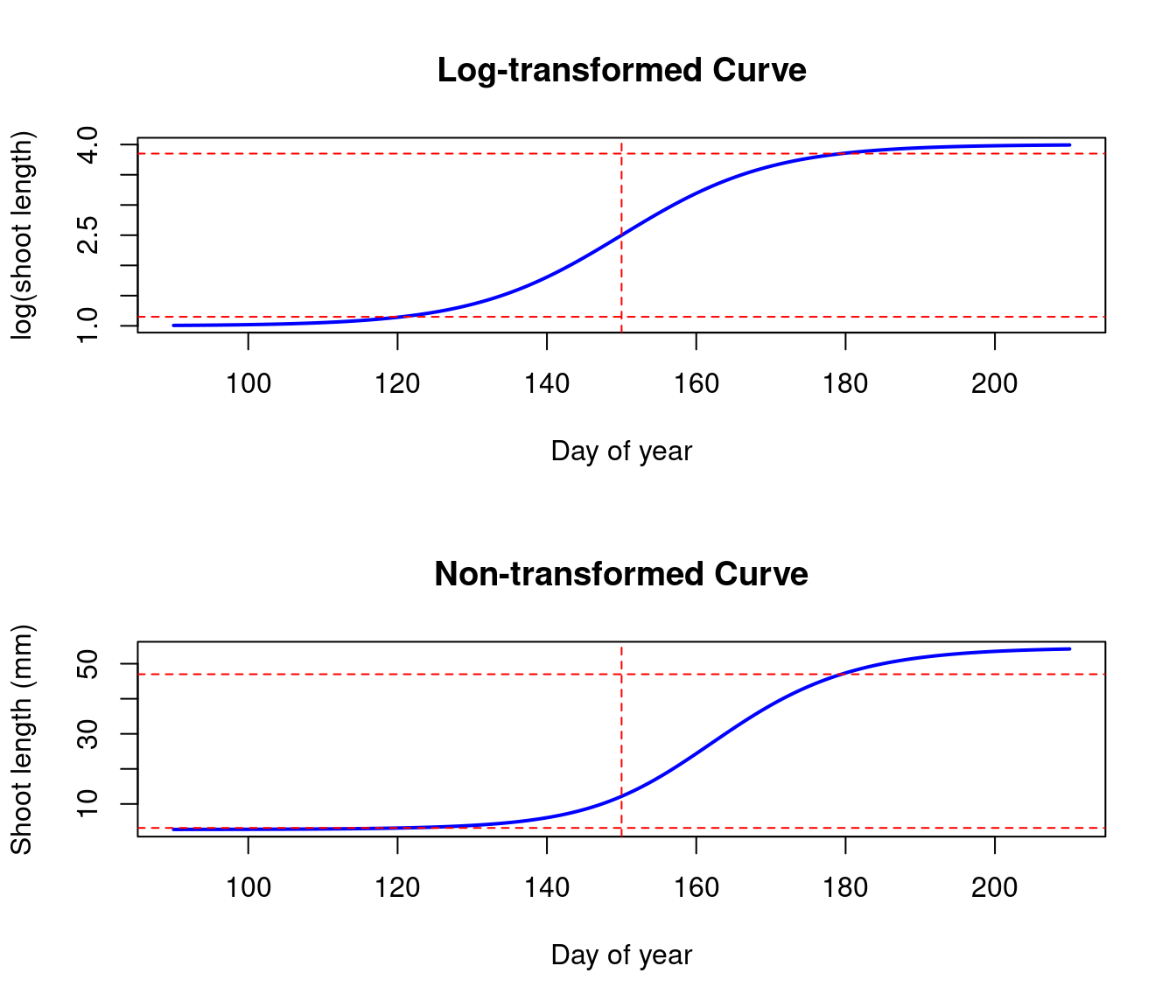
I still recommend fitting the logistic function to the log-transformed data, because of the distribution of errors, the asymmetrical shape of the growth curves before transformation, and that shoot length increase is very likely to be multiplicative, perhaps as shoot cells divide to elongate the whole shoot.

However, this requires us to make some decisions on how to derive ecologically meaningful parameters. We can do either of the following.

1. Stick to the parameters on log scale but be extremely cautious in interpreting them. In this case, all parameters are in the multiplicative sense. We are essentially looking at the phenology and intensity of shoot cell division, instead of the whole shoot growth.
2. Derive the parameters based on the original scale, e.g., using 5% and 95% of the increase in shoot length. The parameters derived with this approach might lack nice statistical properties, or even biological properties if we believe in the multiplicative process, but might align better with what we observe with our eyes.