Background climate
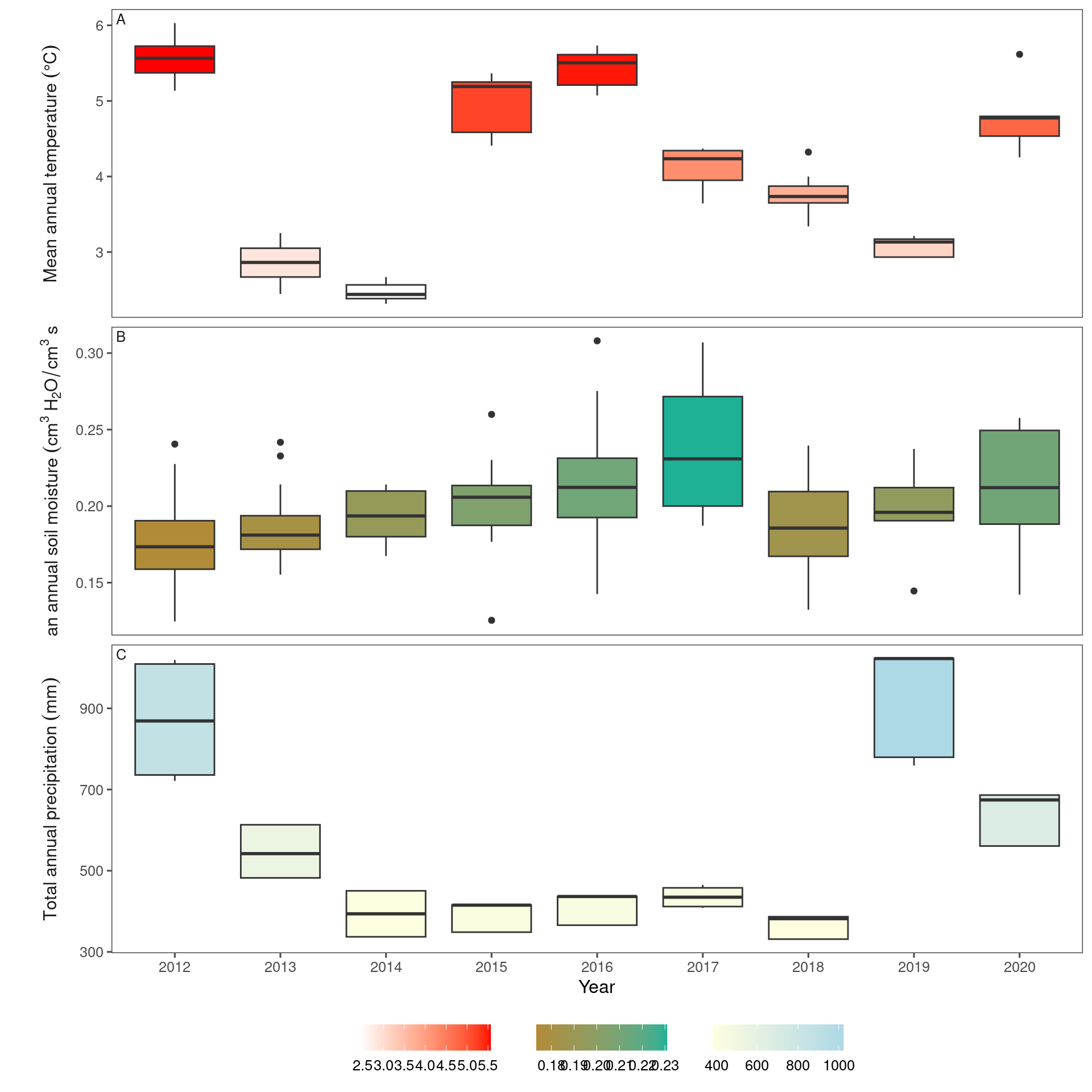
Interannual changes in climatic variables.
dat_climate_annual <- summ_climate_season(dat_climate_daily, date_start = "Jan 1", date_end = "Dec 31", rainfall = 1)
dat_climate_annual_ambient <- calc_climate_ambient(dat_climate_annual, dat_phenophase)

plot_climate_change(dat_climate_annual_ambient, start_year = 2012)
Long-term climate of the two sites.
dat_climate_annual_ambient %>%
  group_by(site) %>%
  filter(year >= 2012) %>%
  summarise(
    temp_mean = mean(temp, na.rm = T),
    mois_mean = mean(mois, na.rm = T),
    prcp_mean = mean(prcp, na.rm = T),
    temp_std = sd(temp, na.rm = T),
    mois_std = sd(mois, na.rm = T),
    prcp_std = sd(prcp, na.rm = T)
  )
## # A tibble: 2 × 7
##   site  temp_mean mois_mean prcp_mean temp_std mois_std prcp_std
##   <chr>     <dbl>     <dbl>     <dbl>    <dbl>    <dbl>    <dbl>
## 1 cfc        4.36     0.196      595.     1.10   0.0214     239.
## 2 hwrc       4.10     0.201      471.     1.16   0.0509     158.
Factorial design
There are still problems with the block and plot IDs.
dat_shoot %>%
  pull(plot) %>%
  unique() %>%
  length()
## [1] 72
dat_shoot %>%
  group_by(site, canopy, heat_name, water_name) %>%
  summarise(
    n_block = n_distinct(block),
    n_plot = n_distinct(plot)
  )
## # A tibble: 18 × 6
## # Groups:   site, canopy, heat_name [12]
##    site  canopy heat_name water_name n_block n_plot
##    <chr> <chr>  <fct>     <fct>        <int>  <int>
##  1 cfc   closed ambient   ambient          3      6
##  2 cfc   closed +1.7 °C   ambient          3      6
##  3 cfc   closed +3.4 °C   ambient          3      6
##  4 cfc   open   ambient   ambient          3      3
##  5 cfc   open   ambient   reduced          3      3
##  6 cfc   open   +1.7 °C   ambient          3      3
##  7 cfc   open   +1.7 °C   reduced          3      3
##  8 cfc   open   +3.4 °C   ambient          3      3
##  9 cfc   open   +3.4 °C   reduced          3      3
## 10 hwrc  closed ambient   ambient          3      6
## 11 hwrc  closed +1.7 °C   ambient          3      6
## 12 hwrc  closed +3.4 °C   ambient          3      6
## 13 hwrc  open   ambient   ambient          3      3
## 14 hwrc  open   ambient   reduced          3      3
## 15 hwrc  open   +1.7 °C   ambient          3      4
## 16 hwrc  open   +1.7 °C   reduced          3      3
## 17 hwrc  open   +3.4 °C   ambient          3      4
## 18 hwrc  open   +3.4 °C   reduced          3      3
dat_shoot %>%
  distinct(site, canopy, heat_name, water_name, block, plot) %>%
  arrange(plot)
## # A tibble: 74 × 6
##    site  canopy heat_name water_name block plot
##    <chr> <chr>  <fct>     <fct>      <chr> <chr>
##  1 cfc   closed +3.4 °C   ambient    a     a1
##  2 cfc   closed +1.7 °C   ambient    a     a2
##  3 cfc   closed ambient   ambient    a     a3
##  4 cfc   closed ambient   ambient    a     a5
##  5 cfc   closed +1.7 °C   ambient    a     a6
##  6 cfc   closed +3.4 °C   ambient    a     a7
##  7 cfc   closed +1.7 °C   ambient    b     b2
##  8 cfc   closed ambient   ambient    b     b3
##  9 cfc   closed +3.4 °C   ambient    b     b4
## 10 cfc   closed +3.4 °C   ambient    b     b5
## # ℹ 64 more rows
Seedling planting
dat_phenophase %>%
  group_by(cohort) %>%
  summarise(n_seedling = n_distinct(barcode)) %>%
  arrange(cohort)
## # A tibble: 7 × 2
##   cohort n_seedling
##    <dbl>      <int>
## 1   2008       2487
## 2   2011         63
## 3   2012       1175
## 4   2013        302
## 5   2014       1791
## 6   2017       1483
## 7   2020         23
dat_phenophase %>%
  mutate(age = year - cohort) %>%
  group_by(barcode) %>%
  summarise(max_age = max(age)) %>%
  pull(max_age) %>%
  summary()
##    Min. 1st Qu.  Median    Mean 3rd Qu.    Max.
##    0.00    2.00    3.00    3.07    4.00   11.00
Goodness-of-fit
dat_shoot_extend <- dat_shoot %>% tidy_shoot_extend()

dat_all <- dat_shoot_extend %>%
  filter(doy > 90, doy <= 210) %>%
  filter(shoot > 0) %>%
  drop_na(barcode) %>%
  group_by(species) %>%
  mutate(group = str_c(site, year, sep = "_") %>% factor() %>% as.integer()) %>% # site-year level random effects
  ungroup() %>%
  tidy_treatment_code()

df_bayes_pred_all <- read_bayes_all(path = "alldata/intermediate/shootmodeling/uni/", full_factorial = T, content = "predict")

# Calculate spearman R^2
(df_R2_species <- inner_join(
  dat_all %>% select(species, site, year, heat_trt, water_trt, canopy_code, doy, obs = shoot),
  df_bayes_pred_all %>% select(species, site, year, heat_trt, water_trt, canopy_code, doy, pred = pred_median)
) %>%
  group_by(species) %>%
  summarise(
    R2 = cor(obs, pred, method = "spearman")^2,
    n = n()
  ) %>%
  arrange(desc(R2)))
## # A tibble: 11 × 3
##    species    R2     n
##    <chr>   <dbl> <int>
##  1 pinba   0.773  8057
##  2 picgl   0.743 10411
##  3 quema   0.720 10366
##  4 pinst   0.706 10288
##  5 betpa   0.698 10433
##  6 abiba   0.691  9974
##  7 aceru   0.668 10352
##  8 rhaca   0.631  7221
##  9 queru   0.623 10296
## 10 poptr   0.593  6715
## 11 acesa   0.585 10418
(df_R2_overall <- inner_join(
  dat_all %>% select(species, site, year, heat_trt, water_trt, canopy_code, doy, obs = shoot),
  df_bayes_pred_all %>% select(species, site, year, heat_trt, water_trt, canopy_code, doy, pred = pred_median)
) %>%
  summarise(
    R2 = cor(obs, pred, method = "spearman")^2,
    n = n()
  ))
## # A tibble: 1 × 2
##      R2      n
##   <dbl>  <int>
## 1 0.709 104531
Report coefficients
df_bayes_all <- read_bayes_all(path = "alldata/intermediate/shootmodeling/uni/", full_factorial = T, derived = T, tidy_mcmc = T) %>%
  tidy_species_name()

df_coef_summ <- summ_mcmc(df_bayes_all)

summ_coef(df_coef_summ, response = "midpoint", covariate = "warming")
## # A tibble: 11 × 10
##    param     species response covariate median lower  upper sig   sign  category
##    <chr>     <fct>   <fct>    <fct>      <dbl> <dbl>  <dbl> <chr> <chr> <fct>
##  1 beta_xmi… queru   midpoint warming    -3.64 -4.56 -2.80  sig   –     negativ…
##  2 beta_xmi… acesa   midpoint warming    -3.25 -4.57 -2.08  sig   –     negativ…
##  3 beta_xmi… quema   midpoint warming    -3.10 -3.82 -2.25  sig   –     negativ…
##  4 beta_xmi… picgl   midpoint warming    -3.08 -4.02 -2.17  sig   –     negativ…
##  5 beta_xmi… pinst   midpoint warming    -3.06 -4.51 -1.82  sig   –     negativ…
##  6 beta_xmi… abiba   midpoint warming    -3.02 -4.40 -1.75  sig   –     negativ…
##  7 beta_xmi… betpa   midpoint warming    -2.79 -4.31 -1.35  sig   –     negativ…
##  8 beta_xmi… rhaca   midpoint warming    -2.65 -4.53 -0.919 sig   –     negativ…
##  9 beta_xmi… pinba   midpoint warming    -2.57 -3.57 -1.54  sig   –     negativ…
## 10 beta_xmi… aceru   midpoint warming    -2.56 -3.65 -1.40  sig   –     negativ…
## 11 beta_xmi… poptr   midpoint warming    -2.47 -5.00  0.444 ns    –     negativ…
# omitting other summarise here
Effects on timing
summ_coef(df_coef_summ, response = "midpoint", covariate = "warming")
summ_coef(df_coef_summ, response = "midpoint", covariate = "warming | closed")
summ_coef(df_coef_summ, response = "start", covariate = "warming")
summ_coef(df_coef_summ, response = "start", covariate = "warming | closed")
summ_coef(df_coef_summ, response = "end", covariate = "warming")
summ_coef(df_coef_summ, response = "end", covariate = "warming | closed")

summ_coef(df_coef_summ, response = "midpoint", covariate = "closed")
summ_coef(df_coef_summ, response = "midpoint", covariate = "drying")
summ_coef(df_coef_summ, response = "midpoint", covariate = "warming x drying")
Effects on pace
summ_coef(df_coef_summ, response = "rate", covariate = "warming")
summ_coef(df_coef_summ, response = "rate", covariate = "warming | closed")
summ_coef(df_coef_summ, response = "duration", covariate = "warming")
summ_coef(df_coef_summ, response = "duration", covariate = "warming | closed")
summ_coef(df_coef_summ, response = "speed", covariate = "warming")
summ_coef(df_coef_summ, response = "speed", covariate = "warminasymptoteg | closed")

summ_coef(df_coef_summ, response = "rate", covariate = "closed")
summ_coef(df_coef_summ, response = "duration", covariate = "closed")
summ_coef(df_coef_summ, response = "speed", covariate = "closed")
Effect on magnitude
summ_coef(df_coef_summ, response = "asymptote", covariate = "warming")
summ_coef(df_coef_summ, response = "asymptote", covariate = "warming | closed")

summ_coef(df_coef_summ, response = "asymptote", covariate = "closed")
summ_coef(df_coef_summ, response = "asymptote", covariate = "drying")