Pre-process data
dat_shoot_extend <- dat_shoot %>% tidy_shoot_extend()

dat_all <- dat_shoot_extend %>%
  filter(doy > 90, doy <= 210) %>%
  filter(shoot > 0) %>%
  drop_na(barcode) %>%
  group_by(species) %>%
  mutate(group = str_c(site, year, sep = "_") %>% factor() %>% as.integer()) %>% # site-year level random effects
  ungroup() %>%
  tidy_treatment_code()
Add climate covariates.
dat_climate_spring <- summ_climate_season(dat_climate_daily, date_start = "Mar 15", date_end = "May 15", rainfall = 1)
dat_climate_spring_ambient <- calc_climate_ambient(dat_climate = dat_climate_spring, dat_phenophase)

dat_climate_spring_diff <- calc_climate_diff(dat_climate = dat_climate_spring, dat_climate_ambient = dat_climate_spring_ambient)

usethis::proj_set(str_c(getwd(), "/phenologyb4warmed/"), force = T)
setwd("phenologyb4warmed/")
usethis::use_data(dat_climate_spring_diff, overwrite = T)
setwd("..")
dat_all_cov <- dat_all %>%
  left_join(dat_climate_spring_diff) %>%
  {
    # Extract only the `center` and `std` attributes
    attributes(.)$center <- attr(dat_climate_spring_diff, "center")
    attributes(.)$sd <- attr(dat_climate_spring_diff, "sd")
    .
  } %>%
  drop_na(delta_temp_std, delta_mois_std)
Summarize treatment effects on temperature and moisture.
dat_climate_spring_diff %>%
  group_by(heat_name, water_name, canopy) %>%
  summarise(
    delta_temp_mean = mean(delta_temp, na.rm = T) %>% signif(3),
    delta_mois_mean = mean(delta_mois, na.rm = T) %>% signif(3),
    delta_temp_sd = sd(delta_temp, na.rm = T) %>% signif(3),
    delta_mois_sd = sd(delta_mois, na.rm = T) %>% signif(3)
  ) %>%
  mutate(
    temp = str_c(delta_temp_mean, " ± ", delta_temp_sd),
    mois = str_c(delta_mois_mean, " ± ", delta_mois_sd)
  ) %>%
  select(heat_name, water_name, canopy, temp, mois) %>%
  arrange(canopy, water_name, heat_name)
## # A tibble: 9 × 5
## # Groups:   heat_name, water_name [6]
##   heat_name water_name canopy temp               mois
##   <fct>     <fct>      <fct>  <chr>              <chr>
## 1 ambient   ambient    open   -3.98e-17 ± 0.0654 4.14e-19 ± 0.00877
## 2 +1.7 °C   ambient    open   0.931 ± 0.55       -0.001 ± 0.0313
## 3 +3.4 °C   ambient    open   1.85 ± 0.844       -0.0104 ± 0.0242
## 4 ambient   reduced    open   0.0861 ± 0.557     -0.00342 ± 0.0264
## 5 +1.7 °C   reduced    open   0.887 ± 0.501      0.00105 ± 0.0312
## 6 +3.4 °C   reduced    open   1.74 ± 0.896       -0.0128 ± 0.0262
## 7 ambient   ambient    closed -6.07e-18 ± 0.145  2.31e-18 ± 0.0212
## 8 +1.7 °C   ambient    closed 1.1 ± 0.513        0.00267 ± 0.0403
## 9 +3.4 °C   ambient    closed 2.12 ± 0.944       -0.00462 ± 0.034
Shoot growth model
Data model
\begin{align*} y_{i,t,s,d} \sim \text{Lognormal}(\mu_{i,t,s,d}, \sigma^2) \end{align*}
Process model
\begin{align*} \mu_{i,t,s,d} &= c+\frac{A_{i,t,s}}{1+e^{-k_{i,t,s}(d-x_{0 i,t,s})}} \newline A_{i,t,s} &= \mu_A + \delta_{A,i}+ \alpha_{A,t,s} \newline x_{0 i,t,s} &= \mu_{x_0} + \delta_{x_0,i}+ \alpha_{x_0,t,s} \newline log(k_{i,t,s}) &= \mu_{log(k)} + \delta_{log(k),i}+ \alpha_{log(k),t,s} \end{align*}
Fixed effects
\begin{align*} \delta_{A,i} &= \beta_{A,1} T_i + \beta_{A,2} \theta_i + \beta_{A,3} T_i \theta_i + \beta_{A,4} C_i + \beta_{A,5} T_i C_i \newline \delta_{x_0,i} &= \beta_{x_0,1} T_i + \beta_{x_0,2} \theta_i + \beta_{x_0,3} T_i \theta_i + \beta_{x_0,4} C_i + \beta_{x_0,5} T_i C_i \newline \delta_{log(k),i} &= \beta_{log(k),1} T_i + \beta_{log(k),2} \theta_i + \beta_{log(k),3} T_i \theta_i + \beta_{log(k),4} C_i + \beta_{log(k),5} T_i C_i \end{align*}
Random effects
\begin{align*} \alpha_{A,t,s} &\sim \text{Normal}(0, \sigma_A^2) \newline \alpha_{x_0,t,s} &\sim \text{Normal}(0, \sigma_{x_0}^2) \newline \alpha_{log(k),t,s} &\sim \text{Normal}(0, \sigma_{log(k)}^2) \end{align*}
Priors
\begin{align*} c &\sim \text{Uniform}(0, 1) \newline \mu_A &\sim \text{Uniform}(1, 6) \newline \beta_A &\sim \text{Multivariate Normal} ( \begin{pmatrix} 0 \newline 0 \newline 0 \newline 0 \newline 0 \newline \end{pmatrix}, \begin{pmatrix} 1 & 0 & 0 & 0 & 0 \newline 0 & 1 & 0 & 0 & 0 \newline 0 & 0 & 1 & 0 & 0 \newline 0 & 0 & 0 & 1 & 0 \newline 0 & 0 & 0 & 0 & 1 \newline \end{pmatrix} )\newline \sigma_A^2 &\sim \text{Truncated Normal}(0, 1, 0, \infty) \newline \mu_{x_0} &\sim \text{Uniform}(120, 180) \newline \beta_{x_0} &\sim \text{Multivariate Normal} ( \begin{pmatrix} 0 \newline 0 \newline 0 \newline 0 \newline 0 \newline \end{pmatrix}, \begin{pmatrix} 100 & 0 & 0 & 0 & 0 \newline 0 & 100 & 0 & 0 & 0 \newline 0 & 0 & 100 & 0 & 0 \newline 0 & 0 & 0 & 100 & 0 \newline 0 & 0 & 0 & 0 & 100 \newline \end{pmatrix} )\newline \sigma_{x_0}^2 &\sim \text{Truncated Normal}(0, 100, 0, \infty) \newline \mu_{log(k)} &\sim \text{Uniform}(-4, -1) \newline \beta_{log(k)} &\sim \text{Multivariate Normal} ( \begin{pmatrix} 0 \newline 0 \newline 0 \newline 0 \newline 0 \newline \end{pmatrix}, \begin{pmatrix} 0.04 & 0 & 0 & 0 & 0 \newline 0 & 0.04 & 0 & 0 & 0 \newline 0 & 0 & 0.04 & 0 & 0 \newline 0 & 0 & 0 & 0.04 & 0 \newline 0 & 0 & 0 & 0 & 0.04 \newline \end{pmatrix} )\newline \sigma_{log(k)}^2 &\sim \text{Truncated Normal}(0, 0.04, 0, \infty) \newline \sigma^2 &\sim \text{Truncated Normal}(0, 1, 0, \infty) \end{align*}
calc_bayes_all(
  data = dat_all_cov,
  independent_priors = F, # do not use species-specific empirical informative priors
  uniform_priors = T, # use uniform priors
  intui_param = F, # regular parameterization with asym, xmid, logk
  continuous_cov = T, # continuous covariates for warming and drying treatments
  num_iterations = 50000,
  nthin = 5,
  path = "alldata/intermediate/shootmodeling/cov/",
  num_cores = 20
)
calc_bayes_derived(path = "alldata/intermediate/shootmodeling/cov/", num_cores = 20)
plot_bayes_all(path = "alldata/intermediate/shootmodeling/cov/", num_cores = 20, continuous_cov = T)
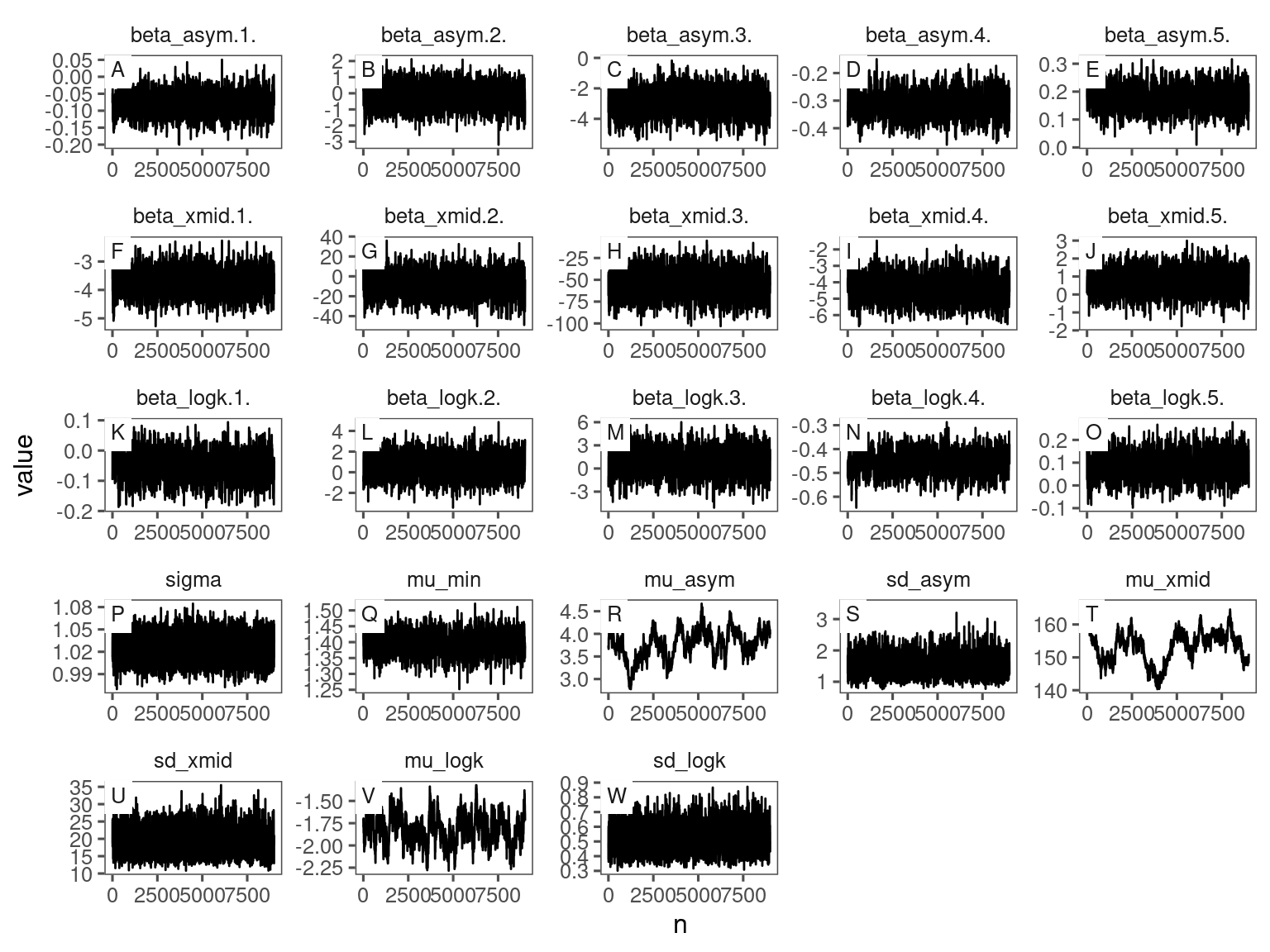
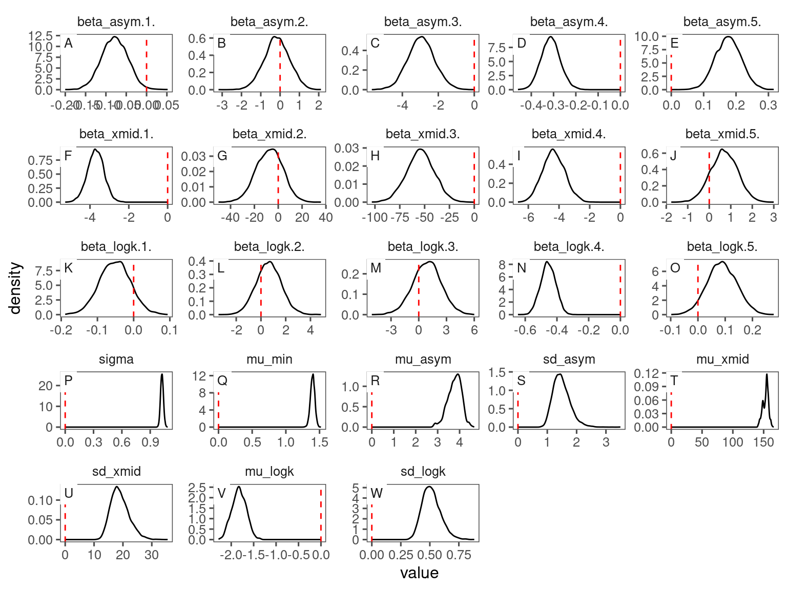
MCMC
df_bayes_all <- read_bayes_all(path = "alldata/intermediate/shootmodeling/cov/", full_factorial = T, derived = F, tidy_mcmc = F)
p_bayes_diagnostics <- plot_bayes_diagnostics(df_MCMC = df_bayes_all %>% filter(species == "queru"), plot_corr = F)
p_bayes_diagnostics$p_MCMC
p_bayes_diagnostics$p_posterior
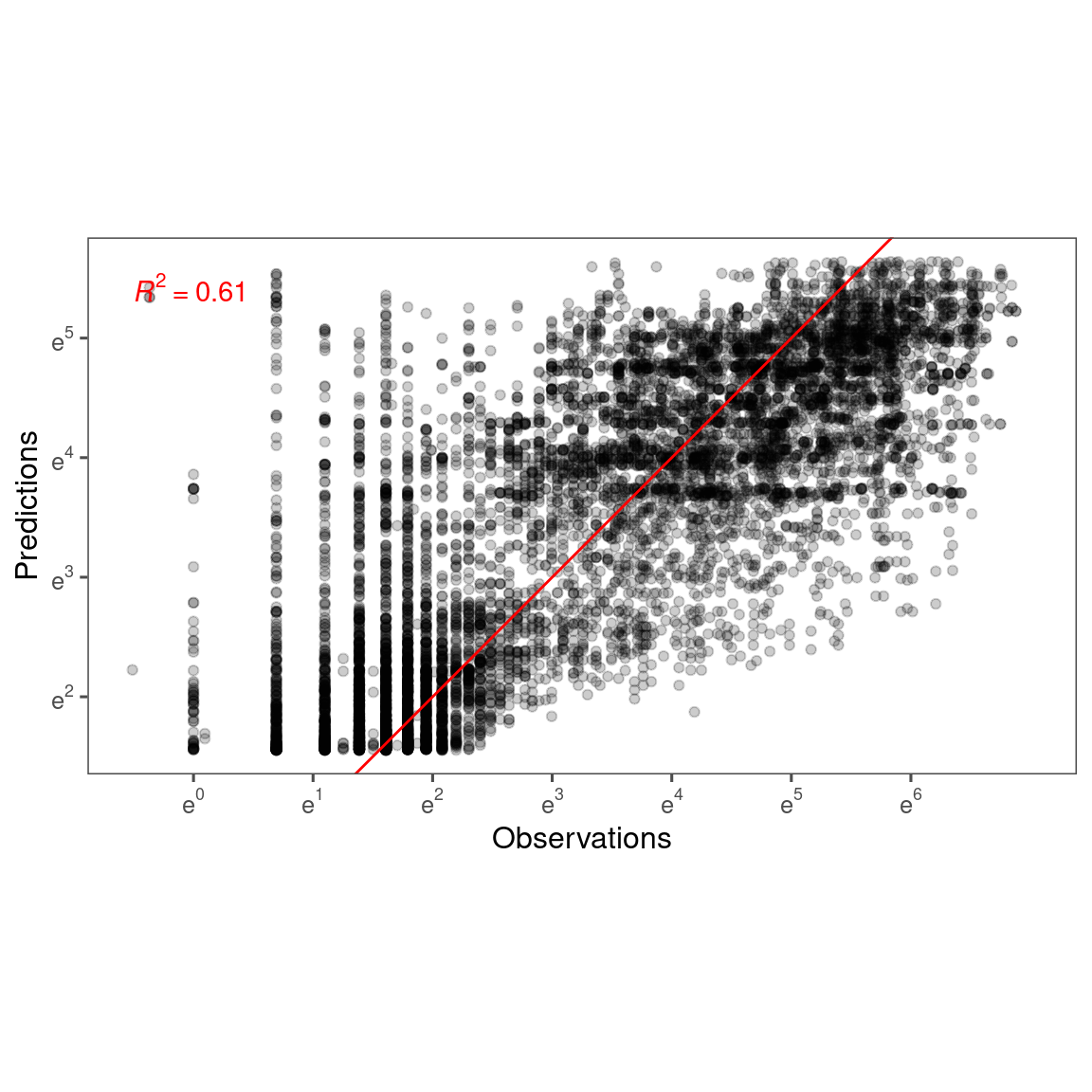
Accuracy
df_bayes_pred_all <- read_bayes_all(path = "alldata/intermediate/shootmodeling/cov/", full_factorial = T, content = "predict")

p_bayes_predict <- plot_bayes_predict(
  data = dat_all %>% filter(species == "queru"),
  data_predict = df_bayes_pred_all %>% filter(species == "queru"),
  vis_log = T,
  vis_ci = T
)
p_bayes_predict$p_accuracy
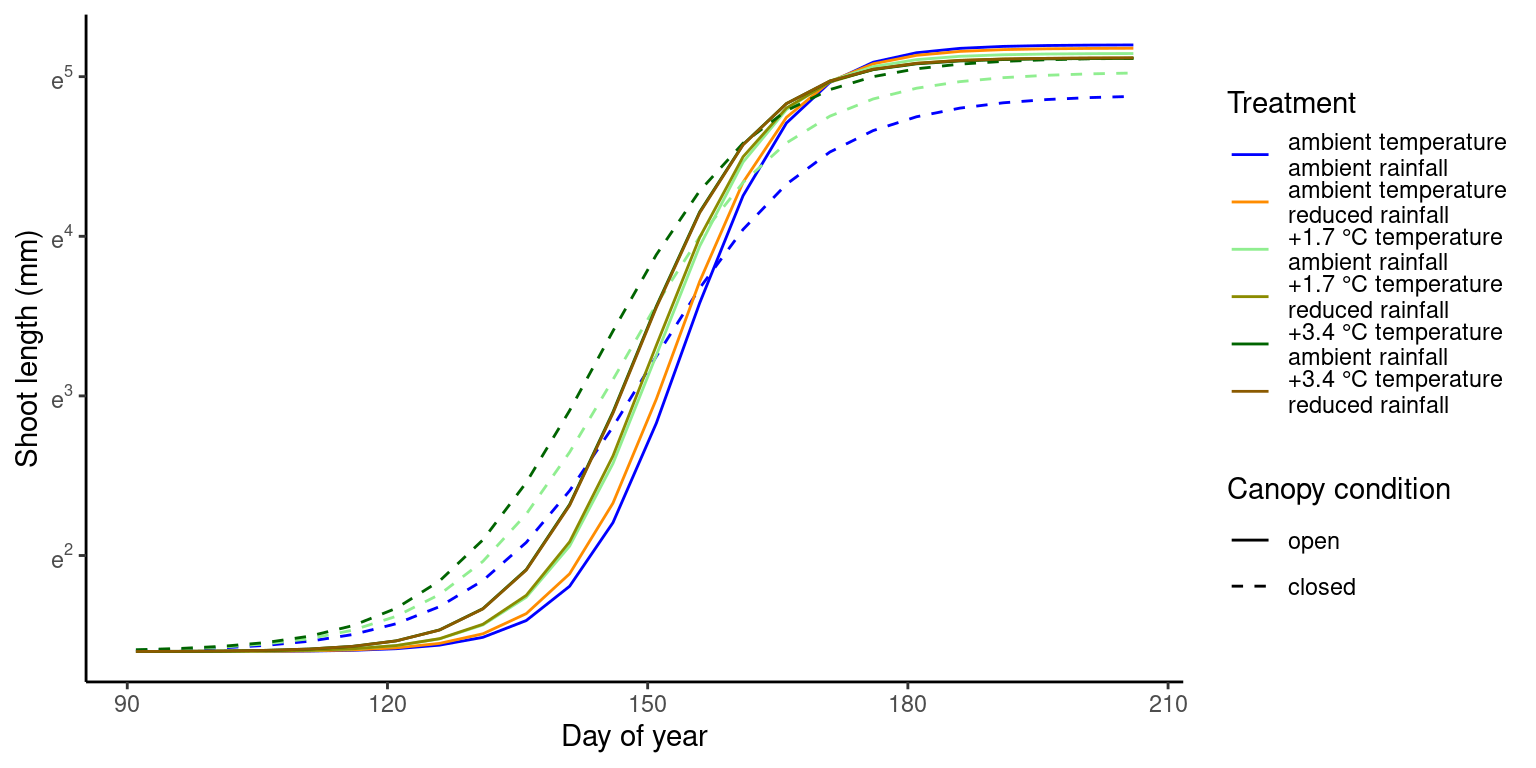
Marginal predictions
df_bayes_pred_marginal_all <- read_bayes_all(path = "alldata/intermediate/shootmodeling/cov/", full_factorial = T, content = "predict_marginal")

p_bayes_predict <- plot_bayes_predict(
  data_predict = df_bayes_pred_marginal_all %>% filter(species == "queru"),
  vis_log = T,
  vis_ci = T
)
p_bayes_predict$p_predict
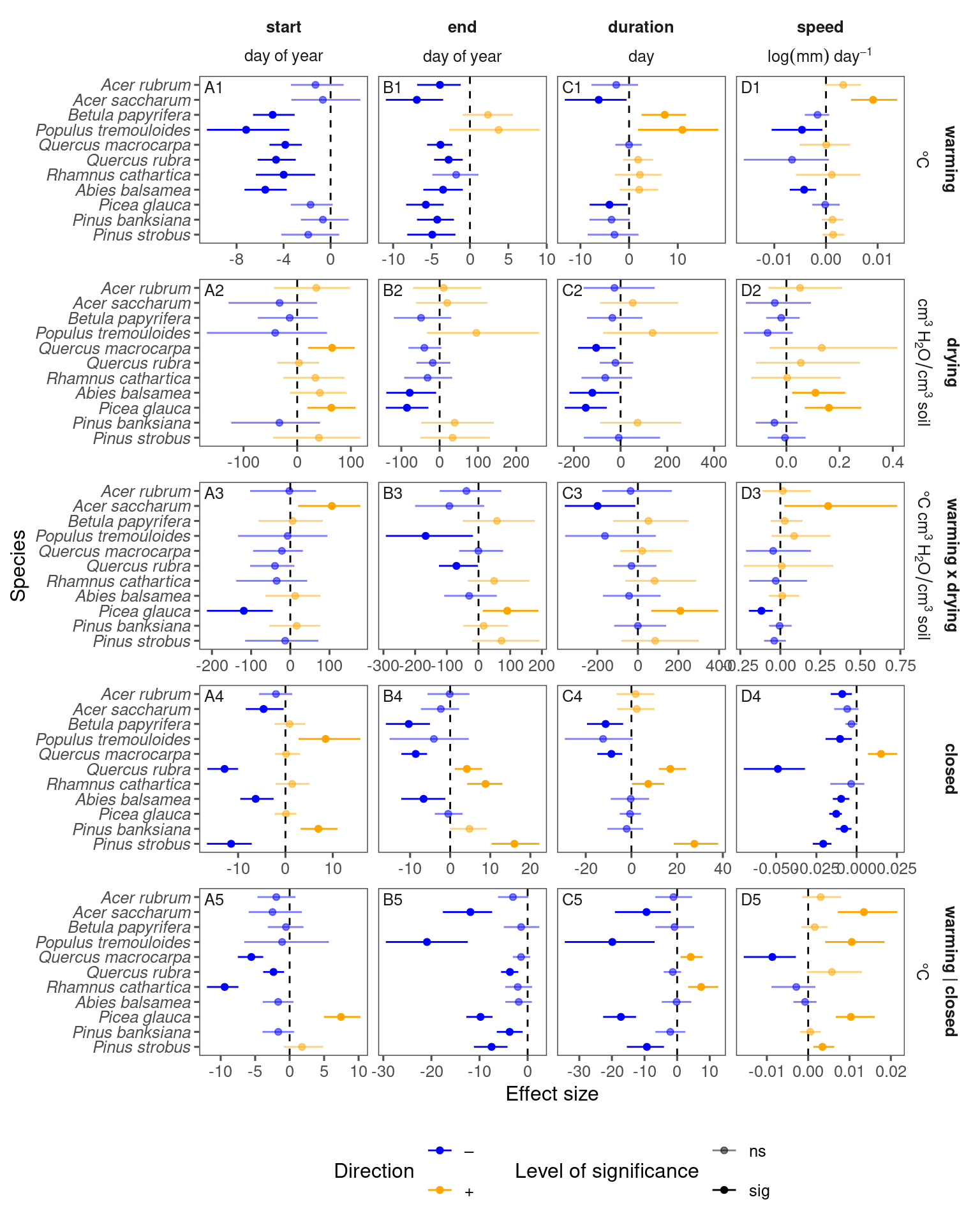
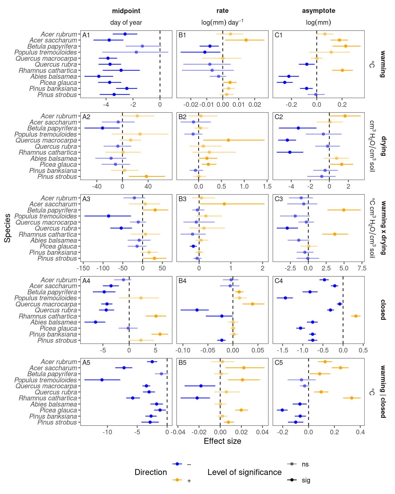
Coefficients
df_bayes_all <- read_bayes_all(path = "alldata/intermediate/shootmodeling/cov/", full_factorial = T, derived = T, tidy_mcmc = T) %>%
  tidy_species_name()
p_bayes_summ <- plot_bayes_summary(df_bayes_all, option = "coef", derived_metric = "no", continuous_cov = T)
p_bayes_summ$p_coef_line
p_bayes_summ <- plot_bayes_summary(df_bayes_all, option = "coef", derived_metric = "only", continuous_cov = T)
p_bayes_summ$p_coef_line