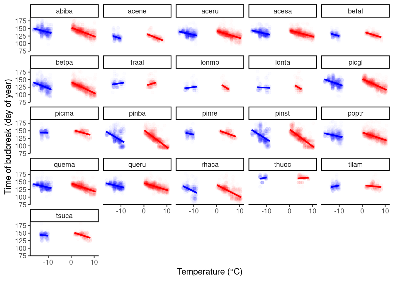
We are curious about how the effects of chilling on time of budbreak can be detected. I did not choose to use process-based models with Growing Degree Days as they have more assumptions and are computationally expensive. I start by comparing the effects of winter warming and spring warming. (Dr. Benjamin Lee recommended this method.)
Temperature is commonly believed to be a key driver of spring phenology. Specifically, cold winter temperatures (chilling) and warm spring temperatures (forcing) interact with each other in determining the timing of leaf-out and flowering. Temperature increases in winter and early spring generally have different impacts on spring phenology. Although higher temperatures in winter may reduce effective chilling accumulation and delay leaf-out and flowering, warmer spring conditions may accelerate the fulfillment of phenological heat requirements, resulting in earlier onset of spring events. Recently, increased scientific interest has focused on the relative importance of chilling and forcing on the timing of spring events. Most studies have identified forcing as the dominant factor governing spring phenology. However, the observed and predicted declines in chilling have increasingly been suggested to be important in determining spring timing. Paper
Calculate phenophase time. Here we only focus on budbreak, which has known hypotheses on chilling effects.
dat_phenophase_time <- dat_phenophase_time_clean %>%
  filter(phenophase == "budbreak") %>%
  group_by(species) %>%
  mutate(group = site %>% factor() %>% as.integer()) %>%
  ungroup() %>%
  mutate(heat_trt = factor(heat_name, levels = c("ambient", "+1.7C", "+3.4C"), labels = c(0, 1, 2)) %>% as.character() %>% as.integer()) %>%
  mutate(water_trt = factor(water_name, levels = c("ambient", "reduced"), labels = c(0, 1)) %>% as.character() %>% as.integer()) %>%
  mutate(canopy_code = factor(canopy, levels = c("open", "closed"), labels = c(0, 1)) %>% as.character() %>% as.integer())
Calculate background climatic variables for all plots (not just ambient).
dat_climate_spring <- summ_climate_season(dat_climate_daily, date_start = "Mar 15", date_end = "May 15", rainfall = 1, group_vars = c("site", "canopy", "heat", "water", "block", "plot", "year")) %>%
  select(site, canopy, heat, water, block, plot, year, spring = temp)

dat_climate_winter <- summ_climate_season(dat_climate_daily, date_start = "Dec 15", start_rollback = 1, date_end = "Feb 15", rainfall = 1, group_vars = c("site", "canopy", "heat", "water", "block", "plot", "year")) %>%
  select(site, canopy, heat, water, block, plot, year, winter = temp)
Join with background climate data.
dat_phenophase_time_cov <- dat_phenophase_time %>%
  left_join(dat_climate_spring) %>%
  left_join(dat_climate_winter) %>%
  group_by(species) %>%
  mutate(group = site %>% factor() %>% as.integer()) %>% # use site as random effects, not site-year
  ungroup()
Exploratory plot.
dat_phenophase_time_cov %>%
  ggplot() +
  geom_point(aes(x = winter, y = doy), col = "blue", alpha = 0.01) +
  geom_smooth(aes(x = winter, y = doy), method = "lm", col = "blue") +
  geom_point(aes(x = spring, y = doy), col = "red", alpha = 0.01) +
  geom_smooth(aes(x = spring, y = doy), method = "lm", col = "red") +
  facet_wrap(. ~ species) +
  labs(
    x = "Temperature (°C)",
    y = "Time of budbreak (day of year)"
  ) +
  theme_classic()

Although there were slight differences in how strongly warming advances budbreak between winter warming and spring warming, there did not seem to be a qualitative difference that points to clear delay of budbreak by a lack of chilling. I did not proceed to fit Bayesian LME.