dat_phenophase_time <- dat_phenophase_time_clean %>%
  mutate(heat_trt = factor(heat_name, levels = c("ambient", "+1.7C", "+3.4C"), labels = c(0, 1, 2)) %>% as.character() %>% as.integer()) %>%
  mutate(water_trt = factor(water_name, levels = c("ambient", "reduced"), labels = c(0, 1)) %>% as.character() %>% as.integer()) %>%
  mutate(canopy_code = factor(canopy, levels = c("open", "closed"), labels = c(0, 1)) %>% as.character() %>% as.integer())
Plot with fewer arrows
dat_phenophase_time_summ <- dat_phenophase_time %>%
  summ_phenophase_time(group_vars = c("site", "canopy", "heat", "heat_name", "water", "water_name", "species", "phenophase", "year")) # ignore block and plot
dat_climate_spring <- summ_climate_season(dat_climate_daily, date_start = "Mar 15", date_end = "May 15", rainfall = 1, group_vars = c("site", "canopy", "heat", "heat_name", "water", "water_name", "year"))

dat_climate_fall <- summ_climate_season(dat_climate_daily, date_start = "Jun 15", date_end = "Sep 15", rainfall = 0, group_vars = c("site", "canopy", "heat", "heat_name", "water", "water_name", "year"))
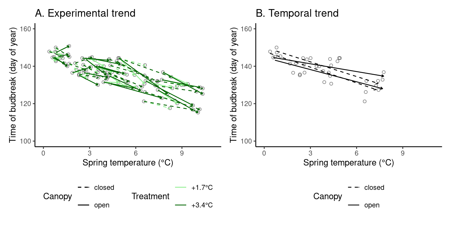
(p_trend1 <- plot_trend(
  dat_phenophase = dat_phenophase_time_summ %>%
    filter(phenophase == "budbreak") %>%
    select(-phenophase) %>%
    filter(species == "queru"),
  dat_climate = dat_climate_spring,
  var = "heat",
  xlim = c(0, 11), ylim = c(100, 160)
))

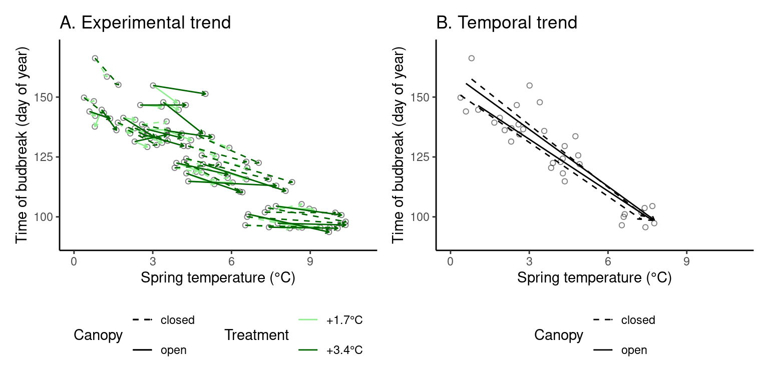
(p_trend2 <- plot_trend(
  dat_phenophase = dat_phenophase_time_summ %>%
    filter(phenophase == "budbreak") %>%
    select(-phenophase) %>%
    filter(species == "pinba"),
  dat_climate = dat_climate_spring,
  var = "heat",
  xlim = c(0, 11), ylim = c(90, 170)
))

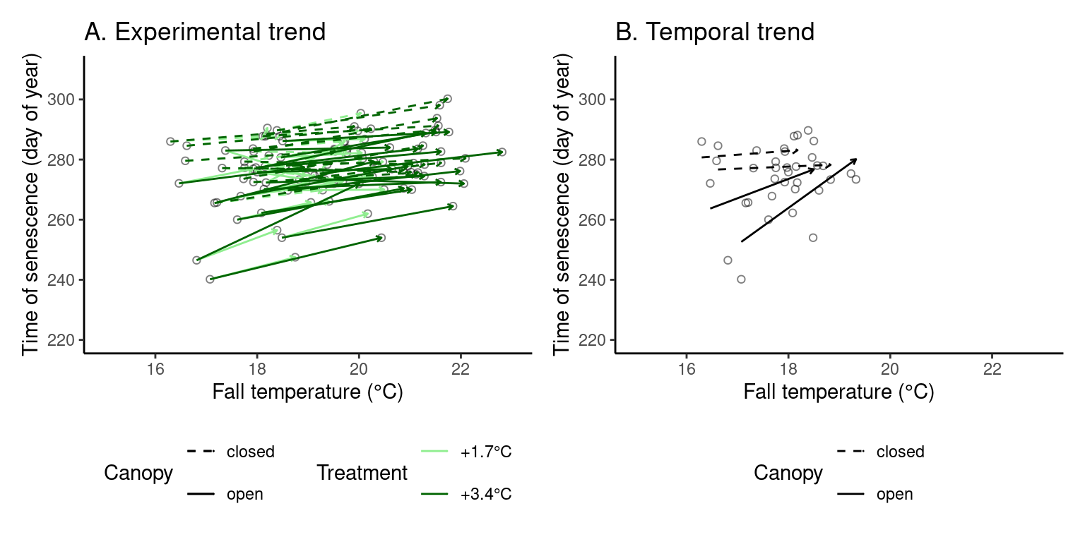
(p_trend3 <- plot_trend(
  dat_phenophase = dat_phenophase_time_summ %>%
    filter(phenophase == "senescence") %>%
    select(-phenophase) %>%
    filter(species == "queru"),
  dat_climate = dat_climate_fall,
  var = "heat",
  xlim = c(15, 23), ylim = c(220, 310),
  xlab = "Fall temperature (°C)", ylab = "Time of senescence (day of year)"
))

Note that the strength of warming treatment, regardless of its effects, seems to be stronger in warmer years.
I only focus on the effects of heat treatment or warming now, because the magnitude of drying treatment was hard to estimate.
Statistical tests
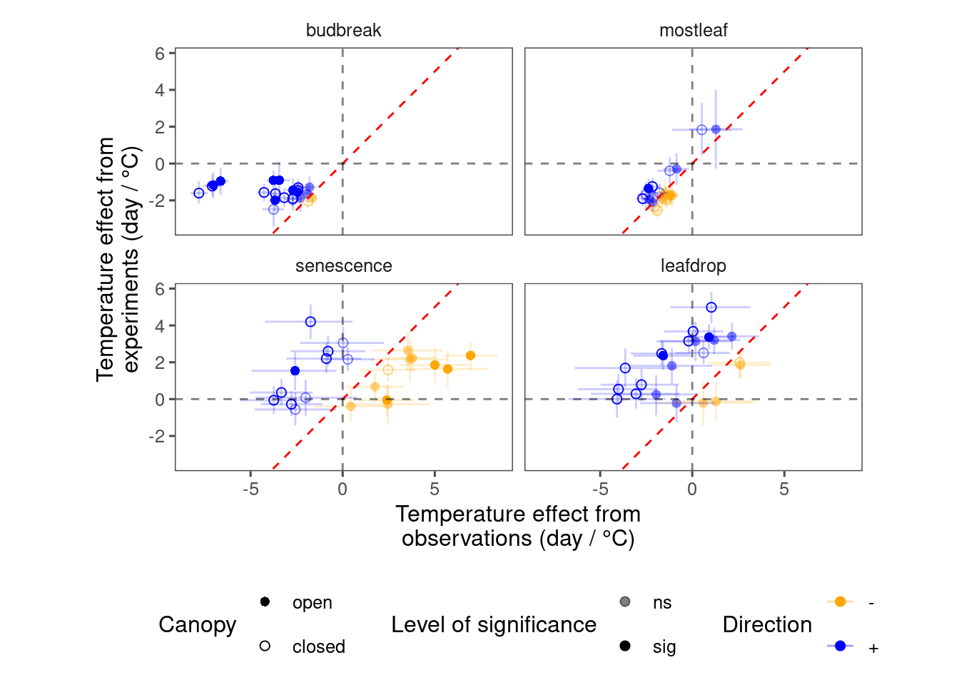
I make use of the results from the Bayesian linear mixed effects model used to infer the effects of treatment and backgroud climate on phenophase status (model version 3). Be careful that coefficients were for scaled background climatic variables. Instead of days degree C or days mm, the units of the coefficients should be days per 1 standard deviation. Reproduce the process of generating climatic variables to find our the scaling factor.
df_plot_ambient <- summ_treatment(dat_phenophase) %>%
  filter(heat_name == "ambient", water_name == "ambient") %>%
  distinct(site, canopy, block, plot)

dat_climate_spring <- summ_climate_season(dat_climate_daily, date_start = "Mar 15", date_end = "May 15", rainfall = 1)
dat_climate_spring_ambient <- dat_climate_spring %>%
  inner_join(df_plot_ambient, by = c("site", "canopy", "block", "plot")) %>%
  group_by(site, canopy, block, year) %>%
  summarise(
    temp = mean(temp),
    mois = mean(mois)
  ) %>%
  ungroup() %>%
  mutate(
    temp_std = scale(temp) %>% as.numeric(),
    mois_std = scale(mois) %>% as.numeric()
  )
temp_sd_spring <- dat_climate_spring_ambient %>% pull(temp) %>% sd()

dat_climate_fall <- summ_climate_season(dat_climate_daily, date_start = "Jun 15", date_end = "Sep 15", rainfall = 0)
dat_climate_fall_ambient <- dat_climate_fall %>%
  inner_join(df_plot_ambient, by = c("site", "canopy", "block", "plot")) %>%
  group_by(site, canopy, block, year) %>%
  summarise(
    temp = mean(temp),
    mois = mean(mois)
  ) %>%
  ungroup() %>%
  mutate(
    temp_std = scale(temp) %>% as.numeric(),
    mois_std = scale(mois) %>% as.numeric()
  )
temp_sd_fall <- dat_climate_fall_ambient %>% pull(temp) %>% sd()
df_lme_spring <- read_bayes_all(path = "alldata/intermediate/phenophase/bg/", season = "spring", full_factorial = T, derived = F, tidy_mcmc = F)
df_compare_trends_spring <- test_compare_trends(df_lme_spring, temp_sd = temp_sd_spring) %>%
  mutate(season = "spring")

df_lme_fall <- read_bayes_all(path = "alldata/intermediate/phenophase/bg/", season = "fall", full_factorial = T, derived = F, tidy_mcmc = F)
df_compare_trends_fall <- test_compare_trends(df_lme_fall, temp_sd = temp_sd_fall) %>%
  mutate(season = "fall")

df_compare_trends <- bind_rows(df_compare_trends_spring, df_compare_trends_fall) %>%
  mutate(season = factor(season, levels = c("spring", "fall"))) %>%
  mutate(response = case_when(
    season == "spring" & response == "start" ~ "budbreak",
    season == "spring" & response == "end" ~ "mostleaf",
    season == "fall" & response == "start" ~ "senescence",
    season == "fall" & response == "end" ~ "leafdrop"
  )) %>%
  mutate(response = factor(response, levels = c("budbreak", "mostleaf", "senescence", "leafdrop")))

plot_trend_compare(df_compare_trends)
