Effects by species and treatments
Make a synthesis figure combining shoot and phenophase responses to treatments.
species <- "queru"
df_shoot <- read_rds(str_c("alldata/intermediate/shootmodeling/uni/", species, "/df_data.rds"))
design <- tidy_species_design(df_shoot)

df_shoot_coef <- read_rds(str_c("alldata/intermediate/shootmodeling/uni/", species, "/df_MCMC.rds")) %>%
  tidy_mcmc(df_shoot) %>%
  summ_mcmc(option = "all", stats = "median") %>%
  filter(is.na(group)) %>%
  select(-group)
df_shoot_pred <- read_rds(str_c("alldata/intermediate/shootmodeling/uni/", species, "/df_pred_marginal.rds"))

df_phenophase_spring <- read_rds(str_c("alldata/intermediate/phenophase/uni/", species, "/spring/df_data.rds"))
df_phenophase_spring_coef <- read_rds(str_c("alldata/intermediate/phenophase/uni/", species, "/spring/df_MCMC.rds")) %>%
  tidy_mcmc(df_phenophase_spring) %>%
  summ_mcmc(option = "all", stats = "median")

df_phenophase_fall <- read_rds(str_c("alldata/intermediate/phenophase/uni/", species, "/fall/df_data.rds"))
df_phenophase_fall_coef <- read_rds(str_c("alldata/intermediate/phenophase/uni/", species, "/fall/df_MCMC.rds")) %>%
  tidy_mcmc(df_phenophase_fall) %>%
  summ_mcmc(option = "all", stats = "median")

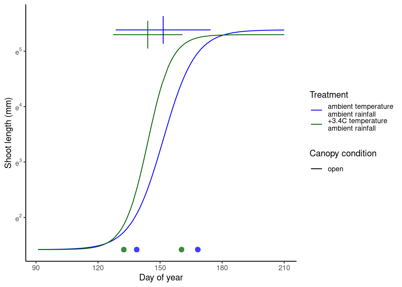
(p_warming <- plot_synthesis_one_trt(df_shoot_pred, df_shoot_coef, df_phenophase_spring_coef, df_phenophase_fall_coef, treatment = "warming", spring_only = T))
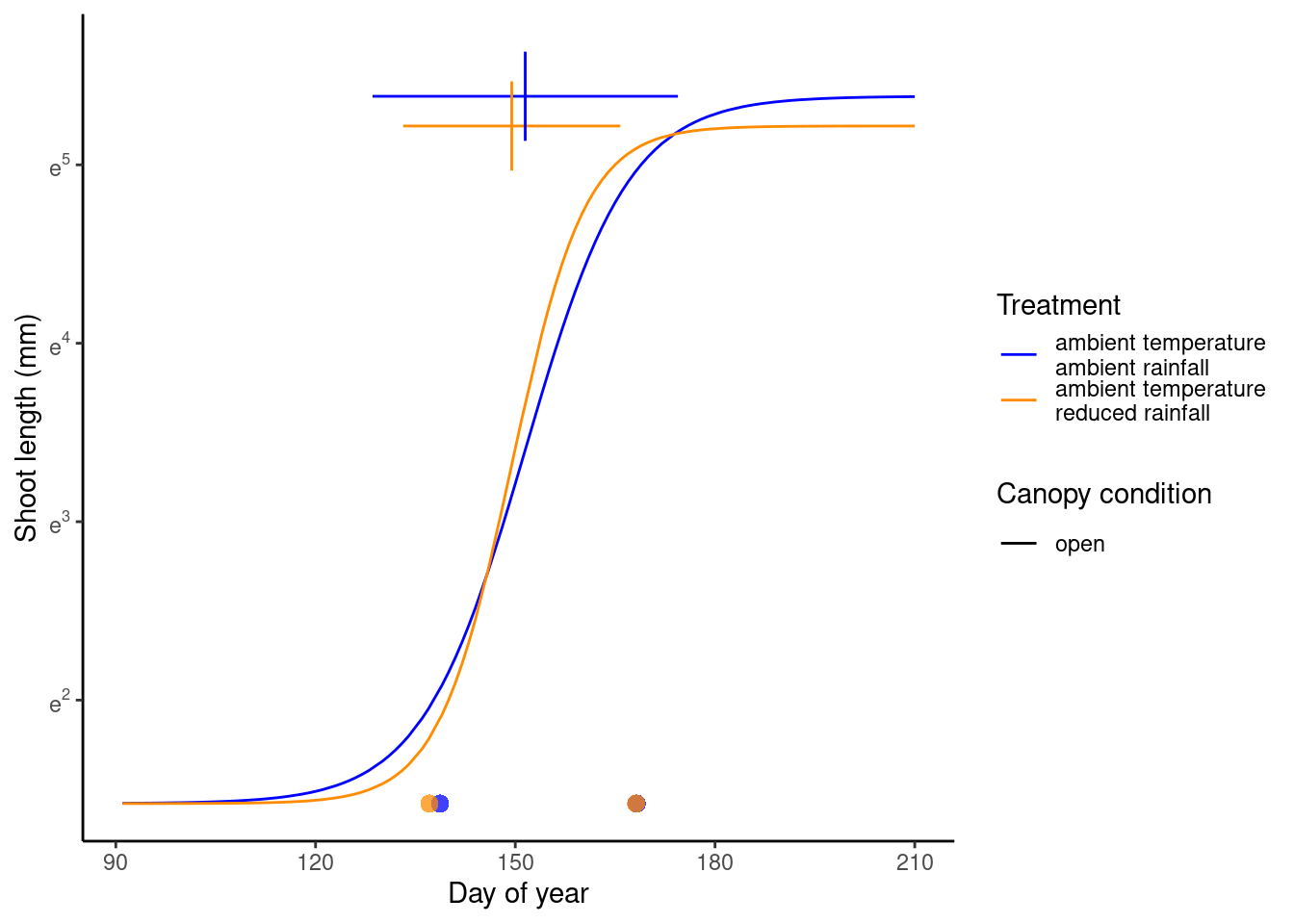
(p_drying <- plot_synthesis_one_trt(df_shoot_pred, df_shoot_coef, df_phenophase_spring_coef, df_phenophase_fall_coef, treatment = "drying", spring_only = T))
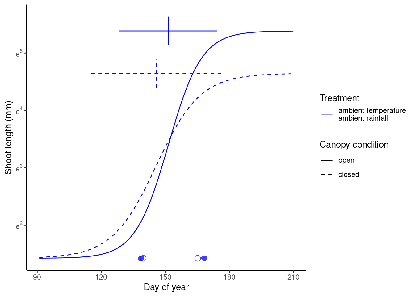
(p_closed <- plot_synthesis_one_trt(df_shoot_pred, df_shoot_coef, df_phenophase_spring_coef, df_phenophase_fall_coef, treatment = "closed", spring_only = T))
plot_synthesis(v_species <- dat_shoot %>% pull(species) %>% unique(), spring_only = T, path = "alldata/output/figures/synthesis/")
Effects across species for each treatment
Make an ordination plot to see patterns of responses in phenophase and shoot growth to a treatment.
df_coef_shoot <- read_bayes_all(path = "alldata/intermediate/shootmodeling/uni/", full_factorial = T, derived = F) %>%
  filter(!is.na(covariate)) %>%
  summ_mcmc(option = "coef", stats = "median")

df_coef_phenophase <- read_bayes_all(path = "alldata/intermediate/phenophase/uni/", season = "spring", full_factorial = T, derived = F) %>%
  filter(!is.na(covariate)) %>%
  summ_mcmc(option = "coef", stats = "median")

plot_ordination(df_coef_shoot, df_coef_phenophase, treatment = "warming")
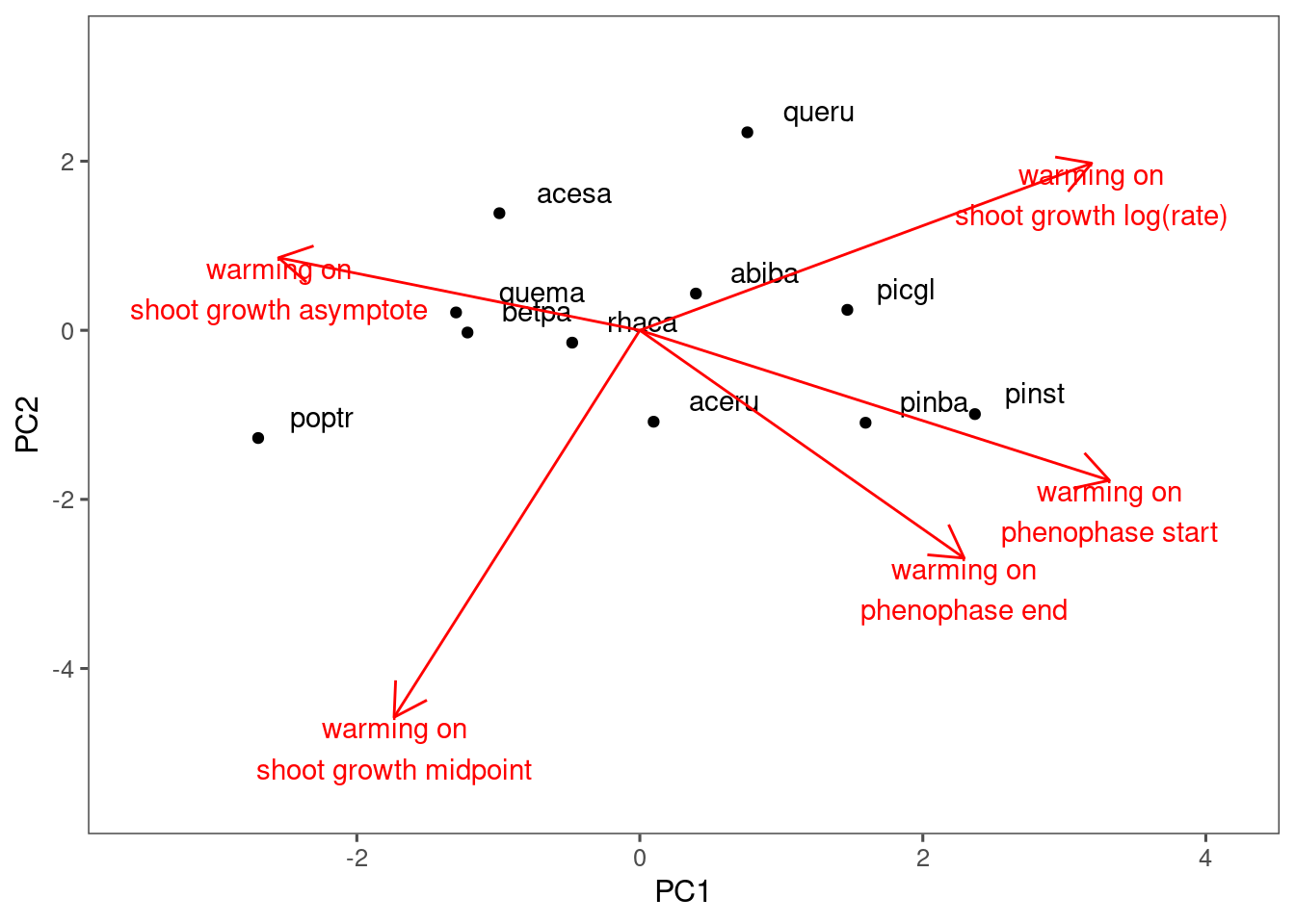 Differentiated mostly by the responses in asymptote. Not much difference in the responses in timings.
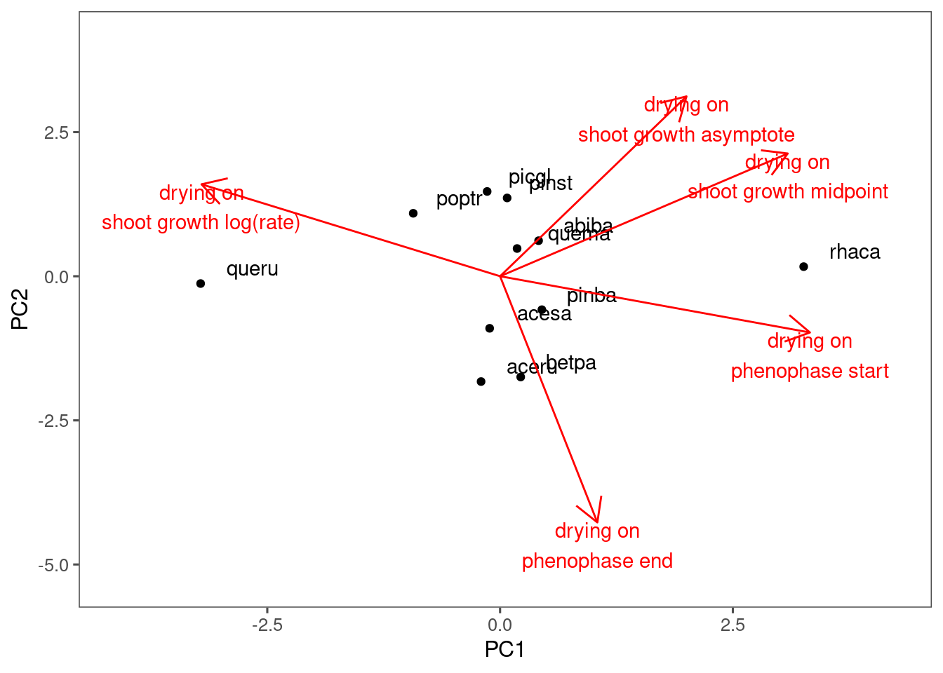
plot_ordination(df_coef_shoot, df_coef_phenophase, treatment = "drying")
plot_ordination(df_coef_shoot, df_coef_phenophase, treatment = "closed")
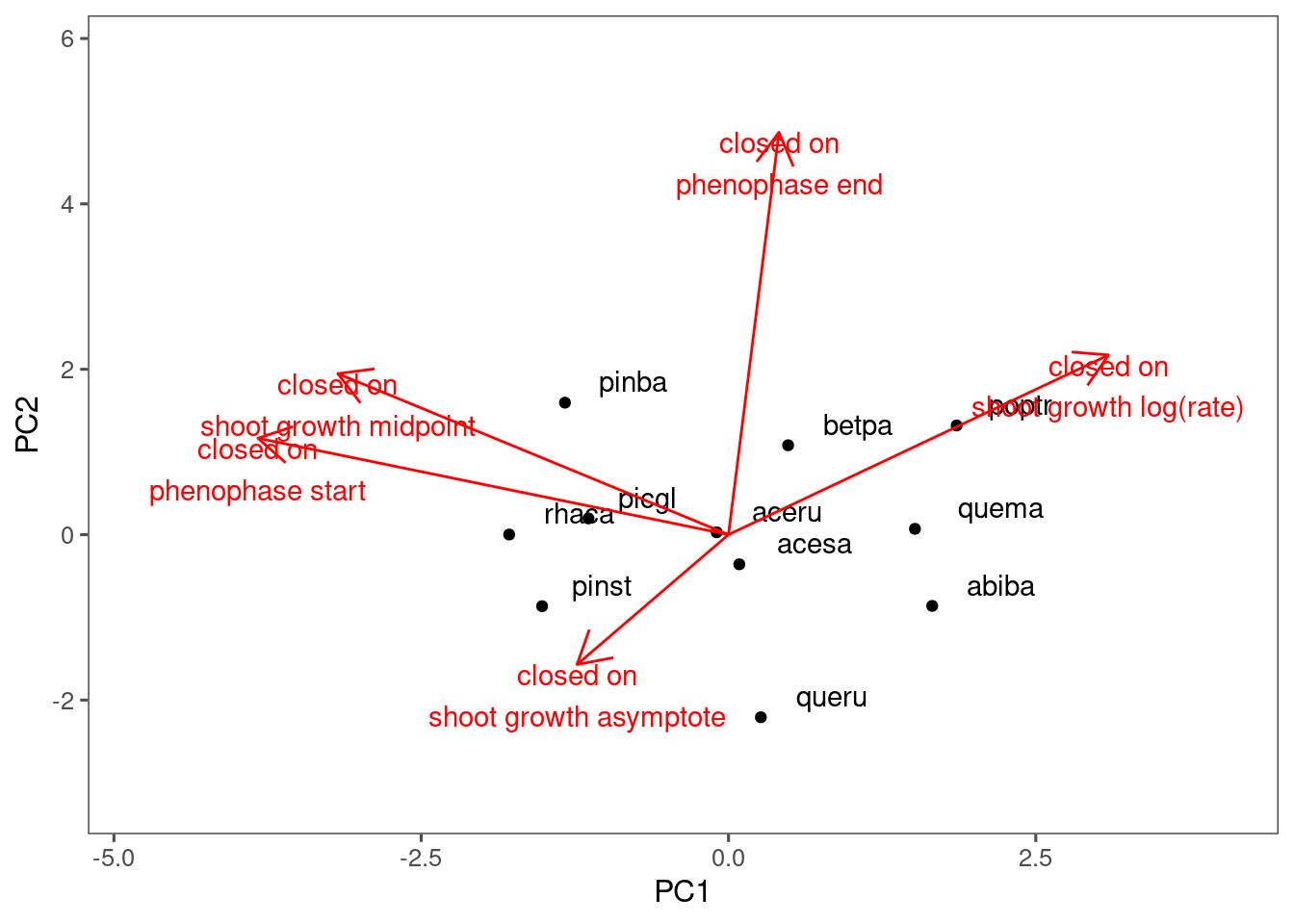
I did not see much clustering in the responses to drying or closed canpopy.