Calculate phenophase time.

dat_phenophase_time <- dat_phenophase_time_clean %>%
  group_by(species) %>%
  mutate(group = str_c(site, year, sep = "_") %>% factor() %>% as.integer()) %>%
  ungroup() %>%
  mutate(heat_trt = factor(heat_name, levels = c("ambient", "+1.7C", "+3.4C"), labels = c(0, 1, 2)) %>% as.character() %>% as.integer()) %>%
  mutate(water_trt = factor(water_name, levels = c("ambient", "reduced"), labels = c(0, 1)) %>% as.character() %>% as.integer()) %>%
  mutate(canopy_code = factor(canopy, levels = c("open", "closed"), labels = c(0, 1)) %>% as.character() %>% as.integer())

Update from the previous analysis, I now use uniform priors for intercepts.

Spring phenophases

Fit Bayesian LME for all species using package brms.

Responses: start (budbreak), end (mostleaf), duration
Covariates: heat, water, heat:water, canopy, heat:canopy
Random-effects: site-year

\begin{aligned} y_{i,t,s} &\sim \mathcal{N}(\mu_{i,t,s}, \sigma^2) \newline \mu_{i,t,s} &= \mu + \beta_1 T_i + \beta_2 D_i + \beta_3 (T_i \times D_i) + \beta_4 C_i + \beta_5 (T_i \times C_i) + \alpha_{t,s} \newline \alpha_{t,s} &\sim \mathcal{N}(0, \tau^2) \newline \newline \mu &\sim \mathcal{U}(1, 180) \newline \beta_{1:5} &\sim \mathcal{N}(0, 4) \newline \sigma &\sim \mathcal{N}(0, 4) \newline \tau &\sim \mathcal{N}(0, 4) \end{aligned}

test_phenophase_lme(data = dat_phenophase_time, path = "alldata/intermediate/phenophase/uni/", season = "spring", chains = 1, iter = 4000, version = 2)
tidy_stanfit_all(path = "alldata/intermediate/phenophase/uni/", season = "spring")
calc_bayes_derived(path = "alldata/intermediate/phenophase/uni/", season = "spring", type = "phenophase", random = F)

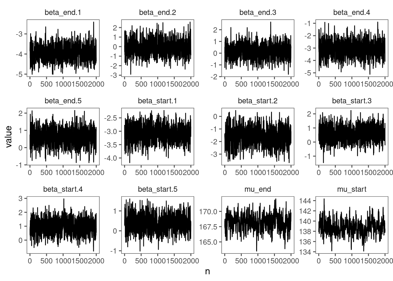
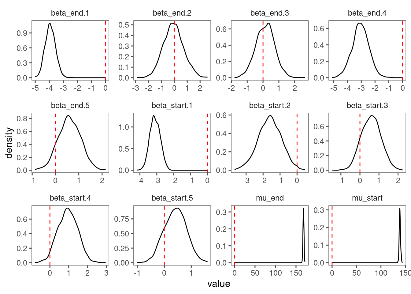
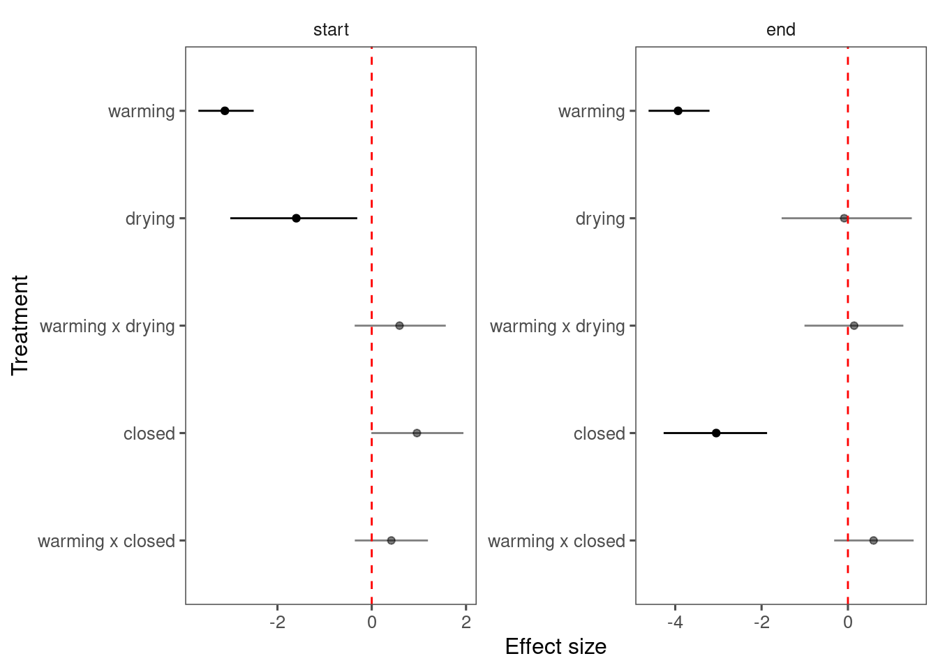
View diagnostics for spring phenology of red oak.

df_lme_all <- read_bayes_all(path = "alldata/intermediate/phenophase/uni/", season = "spring", full_factorial = T, derived = F)

p_lme_diagnostics <- plot_bayes_diagnostics(df_MCMC = df_lme_all %>% filter(species == "queru"), plot_corr = F)
p_lme_diagnostics$p_MCMC

p_lme_diagnostics$p_posterior

p_lme_diagnostics$p_coefficient

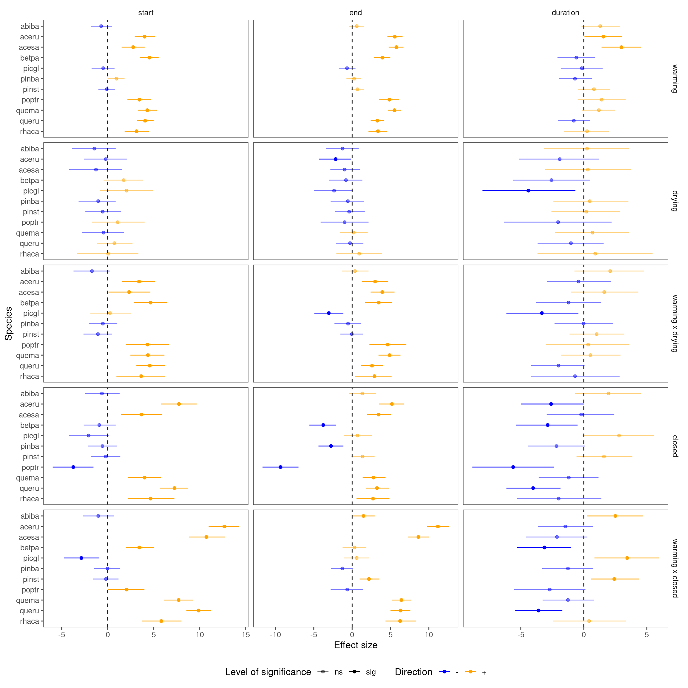
Summarize results for all species.

df_lme_all_derived <- read_bayes_all(path = "alldata/intermediate/phenophase/uni/", season = "spring", full_factorial = T, derived = T)

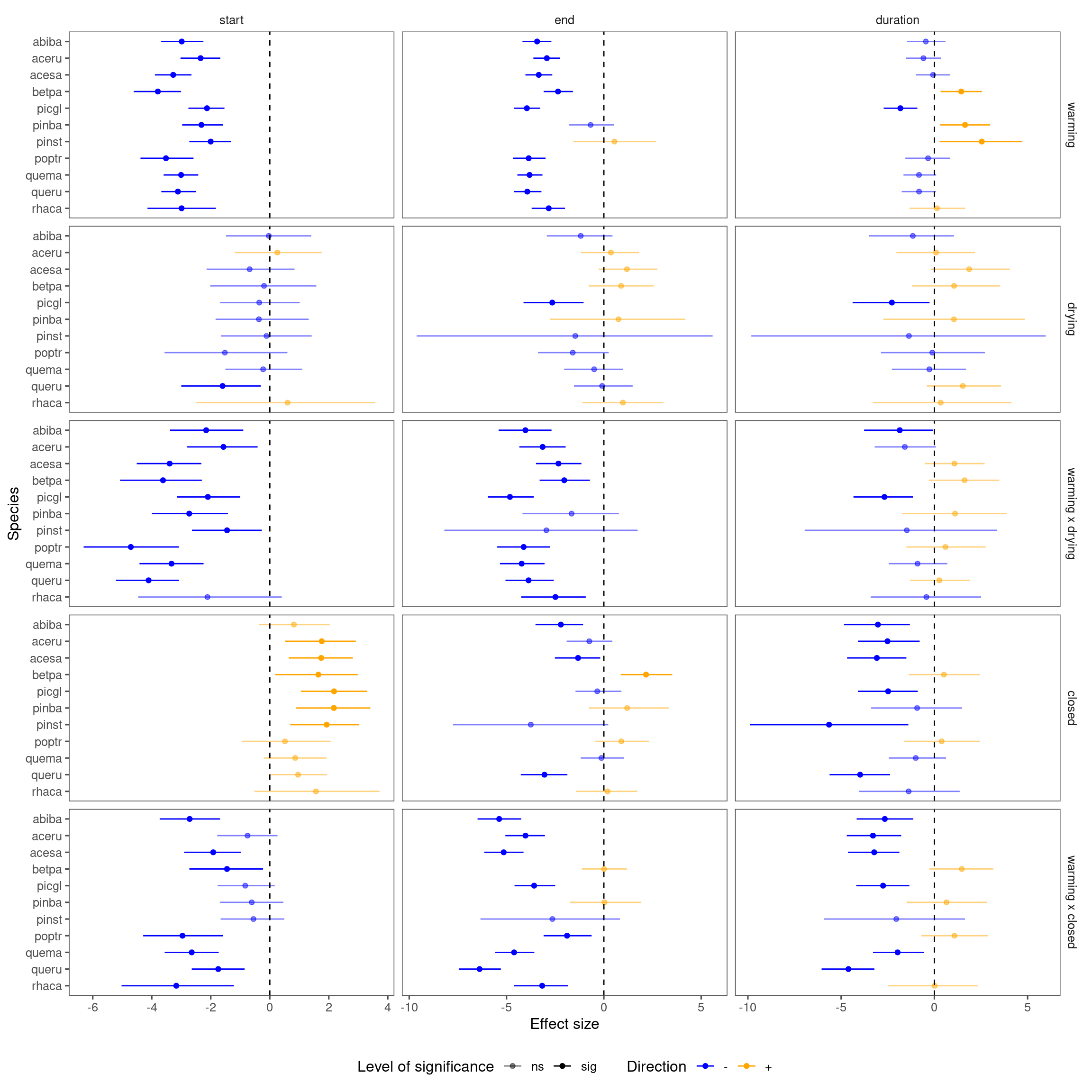
p_lme_summ <- plot_bayes_summary(df_lme_all_derived, plot_corr = F)
p_lme_summ$p_coef_line

Compare with shoot growth results

df_bayes_all_derived <- read_bayes_all(path = "alldata/intermediate/shootmodeling/all/", full_factorial = T, derived = T)
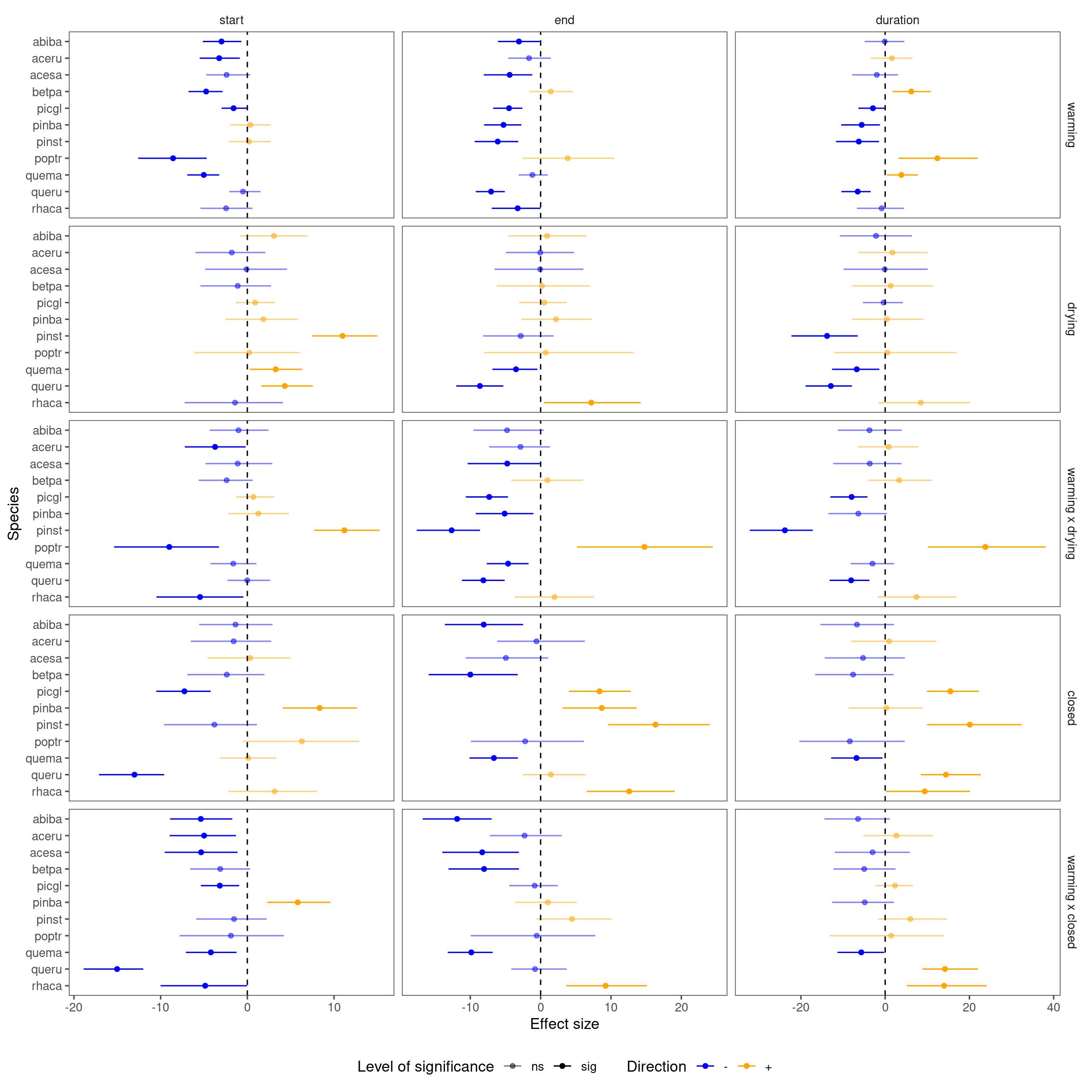
p_bayes_summ_derived <- plot_bayes_summary(df_bayes_all_derived, plot_corr = F, subset = T)
p_bayes_summ_derived$p_coef_line

Fall phenophases

Fit Bayesian LME for each species using package brms.

Responses: start (senescence), end (leafdrop), duration
Covariates: heat, water, heat:water, canopy, heat:canopy
Random-effects: site-year

test_phenophase_lme(data = dat_phenophase_time, path = "alldata/intermediate/phenophase/uni/", season = "fall", chains = 1, iter = 4000)
tidy_stanfit_all(path = "alldata/intermediate/phenophase/uni/", season = "fall")
calc_bayes_derived(path = "alldata/intermediate/phenophase/uni/", season = "fall", type = "phenophase", random = F) # derived interactive effects

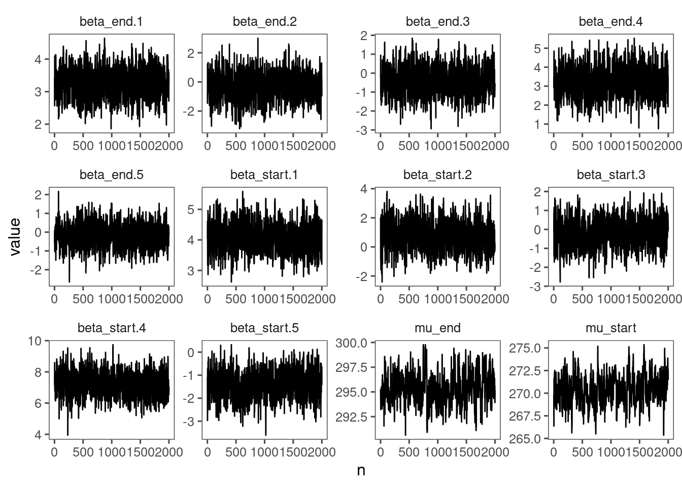
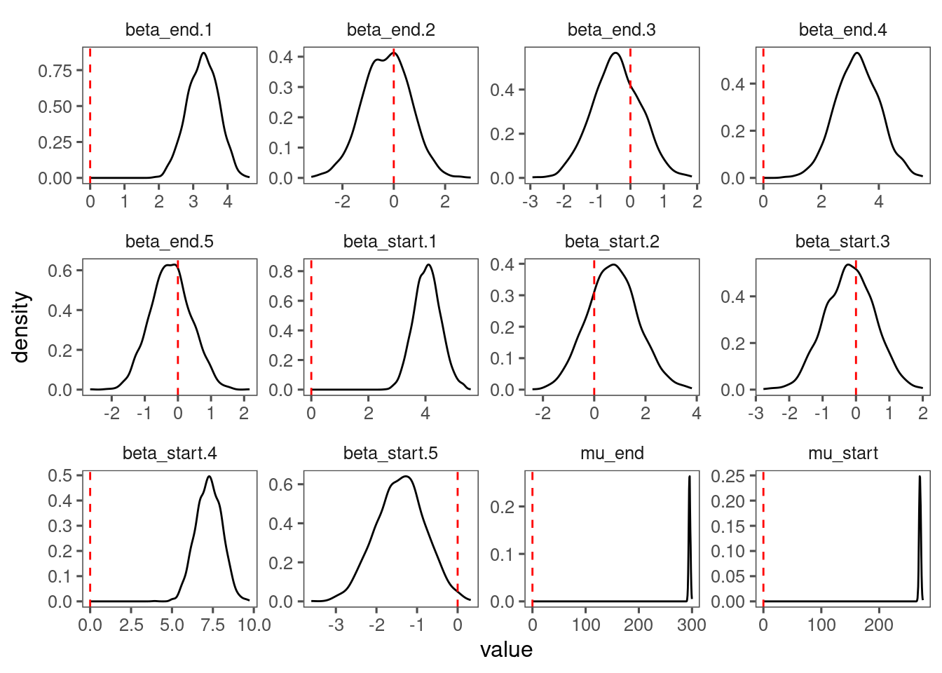
View diagnostics for fall phenology of red oak.

df_lme_all <- read_bayes_all(path = "alldata/intermediate/phenophase/uni/", season = "fall", full_factorial = T, derived = F)

p_lme_diagnostics <- plot_bayes_diagnostics(df_MCMC = df_lme_all %>% filter(species == "queru"), plot_corr = F)
p_lme_diagnostics$p_MCMC

p_lme_diagnostics$p_posterior

p_lme_diagnostics$p_coefficient

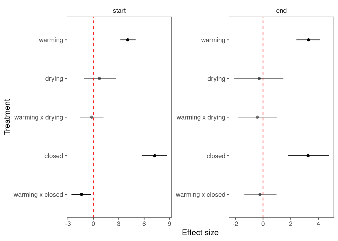
Summarize results for each species.

df_lme_all_derived <- read_bayes_all(path = "alldata/intermediate/phenophase/uni/", season = "fall", full_factorial = T, derived = T)

p_lme_summ <- plot_bayes_summary(df_lme_all_derived, plot_corr = F)
p_lme_summ$p_coef_line

Effects on phenophase 2

Spring phenophases

Compare with shoot growth results

Fall phenophases