This update is focused on data processing, priors, reparameterization, and visualization.
Filling in censored data
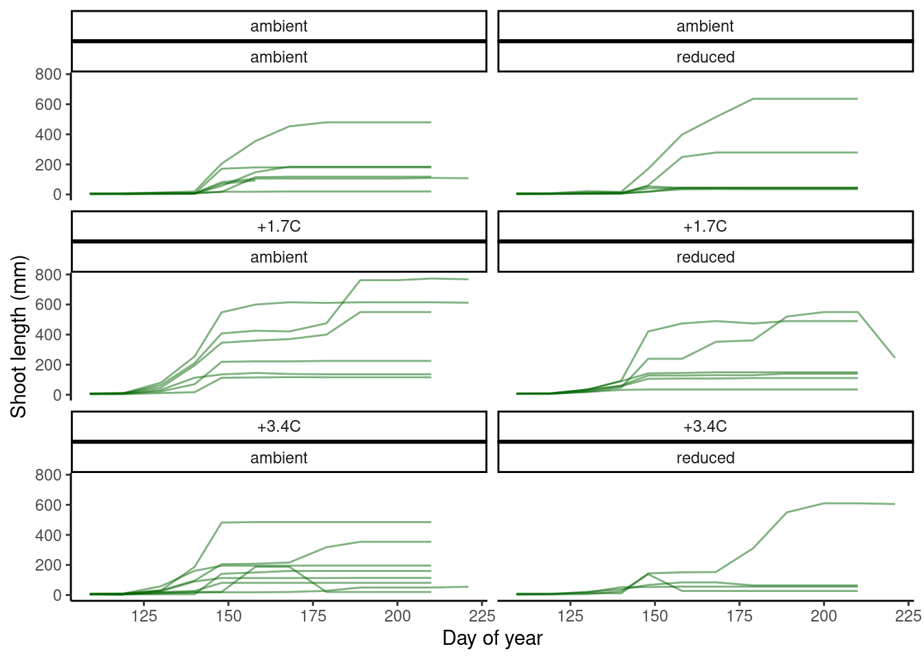
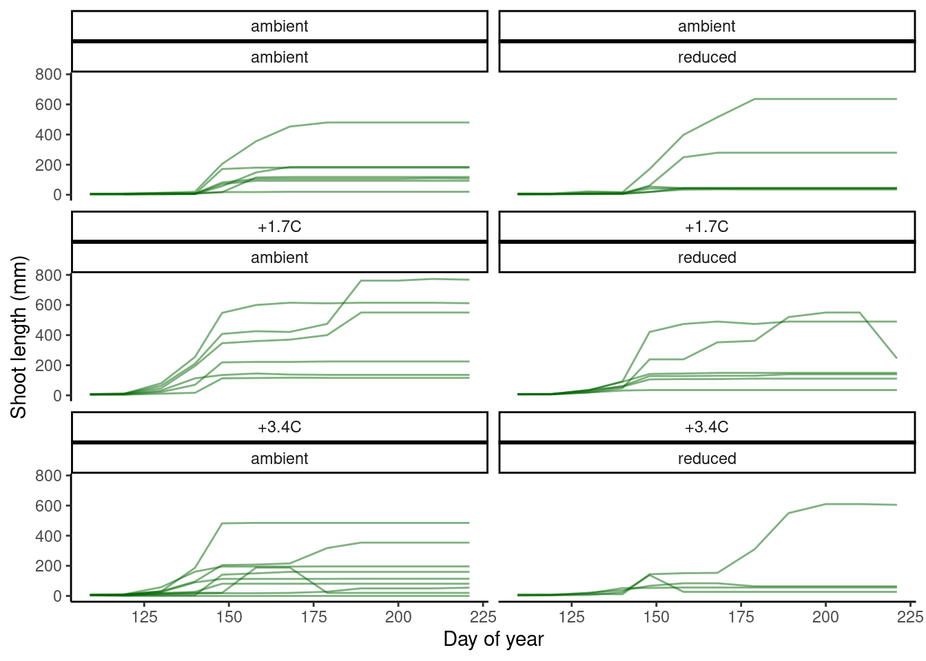
For each individual, shoot measurements stop after the shoot length plateaus. Now I fill in the censored data after sampling stopped with the last observed shoot length. I make sure each site and year have the same end date of sampling.
Note that there are also NAs or inconsistent start dates. I did not fill those in.
# dat_shoot <- tidy_shoot(extend = F)
plot_shoot(dat_shoot %>% filter(year == 2016, site == "hwrc"), speciesoi = "queru")
dat_shoot_extend <- tidy_shoot(extend = T)
plot_shoot(dat_shoot_extend %>% filter(year == 2016, site == "hwrc"), speciesoi = "queru")
dat_shoot_extend_cov <- tidy_shoot(extend = T, covariate = T)
(Deprecated) Making closed canopy the baseline and open canopy a treatment
I attempted to change the coding of the closed and open canopy conditions to make closed canopy the baseline and infer the effects of open canopy. Thought it might be useful for inference of the effects of canopy opening on phenology.
However, because closed canopy does not have drying treatment, it would disrupt the full factorial design and make the previously designed interaction terms difficult to infer.
Decided to keep open canopy as a baseline.
dat_all <- dat_shoot_extend_cov %>%
  filter(doy > 90, doy <= 210) %>%
  filter(shoot > 0) %>%
  drop_na(barcode) %>%
  group_by(species) %>%
  mutate(group = str_c(site, year, sep = "_") %>% factor() %>% as.integer()) %>%
  ungroup() %>%
  mutate(heat_trt = factor(heat_name, levels = c("ambient", "+1.7C", "+3.4C"), labels = c(0, 1, 2)) %>% as.character() %>% as.integer()) %>%
  mutate(water_trt = factor(water_name, levels = c("ambient", "reduced"), labels = c(0, 1)) %>% as.character() %>% as.integer()) %>%
  mutate(canopy_code = factor(canopy, levels = c("open", "closed"), labels = c(0, 1)) %>% as.character() %>% as.integer())
(Deprecated) Setting independent priors for each species
In the previous version, models for all species shared the same priors. This may lead to built-in correlation of parameters among species. I tried to use uniform priors to fit an exploratory model for each species using data from the control, and use the mean and sd of inferred min, start, end, and speed in priors for mu_min, mu_start, mu_end, and mu_speed, respectively.
dat_14 <- dat_all %>%
  filter(species == "queru")
df_MCMC_14 <- calc_bayes_fit(
  data = dat_14 %>%
    filter(
      canopy == if_else("closed" %in% (dat_14 %>% pull(canopy) %>% unique()), "closed", "open"),
      heat == "_",
      water == "_"
    ) %>%
    mutate(tag = "training"),
  version = 14 # uniform prior, reparameterized
)
write_rds(df_MCMC_14, "alldata/intermediate/shootmodeling/df_MCMC_14.rds")
df_MCMC_14 <- read_rds("alldata/intermediate/shootmodeling/df_MCMC_14.rds")

mat_prior <- summ_mcmc(df_MCMC_14,
  option = "all",
  stats = "mean"
) %>%
  column_to_rownames(var = "param") %>%
  as.matrix()

mat_prior
##               mean          sd
## min     1.49398157 0.074656741
## start 121.98624641 3.051821367
## end   168.89969484 2.910885103
## speed   0.05330639 0.005509204
## sigma   1.09351416 0.043747358
Although these empirical informative priors are close to the informative priors I previously prescribed, this is not a standard practice because 1) I was using the same data twice and 2) I used a different model for exploration from the model for inference.
Uniform prior instead of informative normal priors
I also tried the same broad uniform priors for all species, now coded in Models 18, 19, 20.
dat_18 <- dat_all %>%
  filter(species == "queru")
df_MCMC_18 <- calc_bayes_fit(
  data = dat_18 %>% mutate(tag = "training"),
  version = 18, # with uniform priors, regular parameterization
  num_iterations = 50000,
  nthin = 5
)
write_rds(df_MCMC_18, "alldata/intermediate/shootmodeling/df_MCMC_18.rds")
df_MCMC_18 <- read_rds("alldata/intermediate/shootmodeling/df_MCMC_18.rds") %>% tidy_mcmc(dat_18)
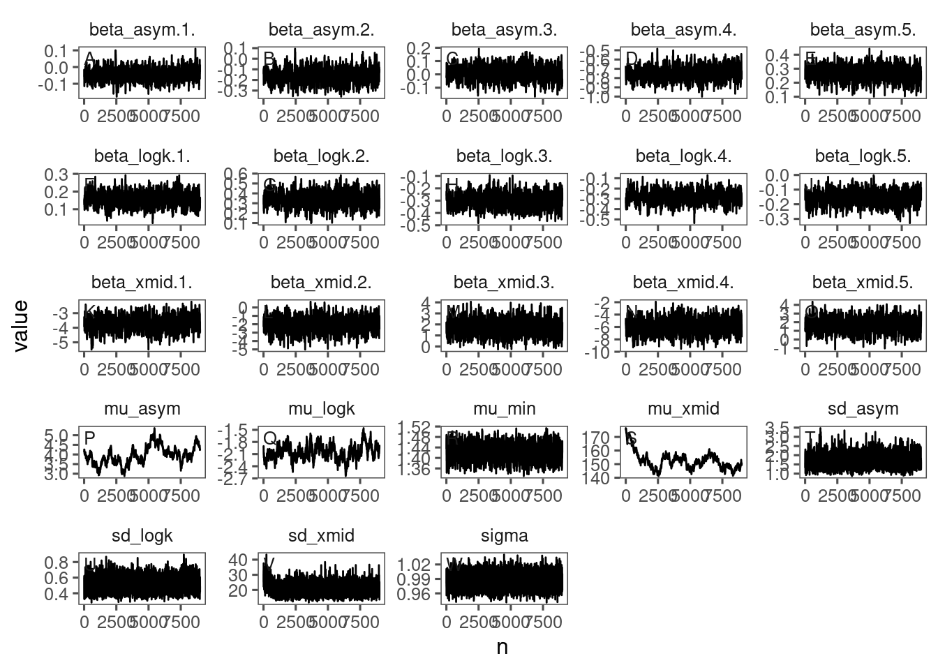
p_bayes_diagnostics <- plot_bayes_diagnostics(df_MCMC = df_MCMC_18)
p_bayes_diagnostics$p_MCMC
p_bayes_diagnostics$p_coefficient
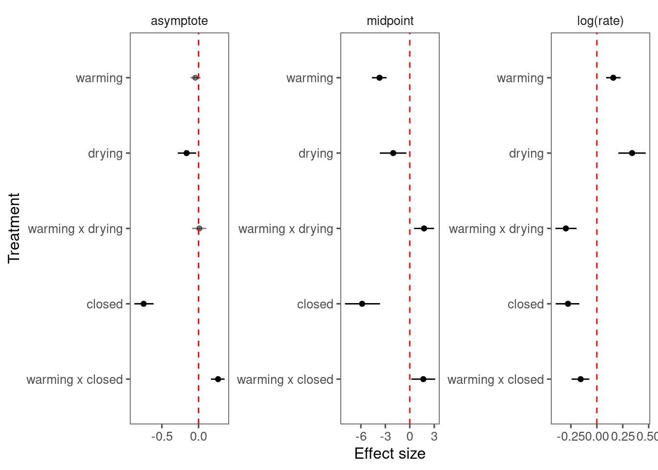
Mixing and inference very similar to those from normal priors. Can consider.
(Deprecated) Reparameterizing with start, end, and speed
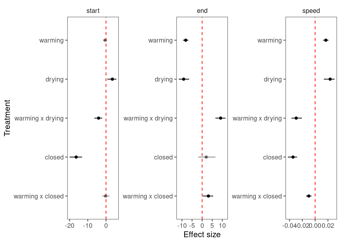
In previous models, the logistic function was parameterized with min, asym, xmid, and logk. I tried to reparameterize the logistic function with min, start, end, and speed. This was intended to make the inference more interpretable and to break the built-in correlations between treatment effects on the derived parameters e.g., start and end, duration and speed.
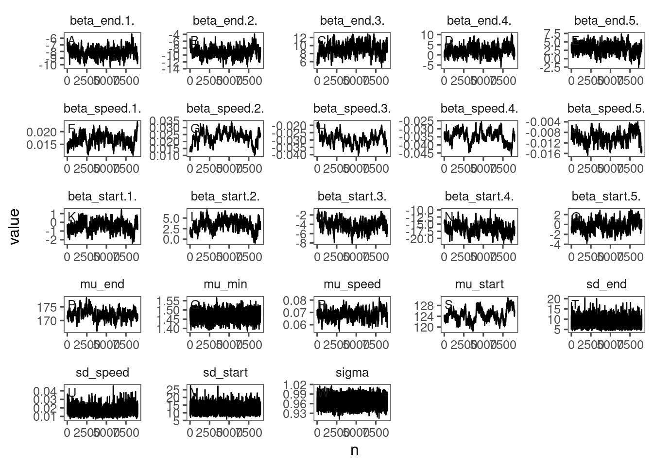
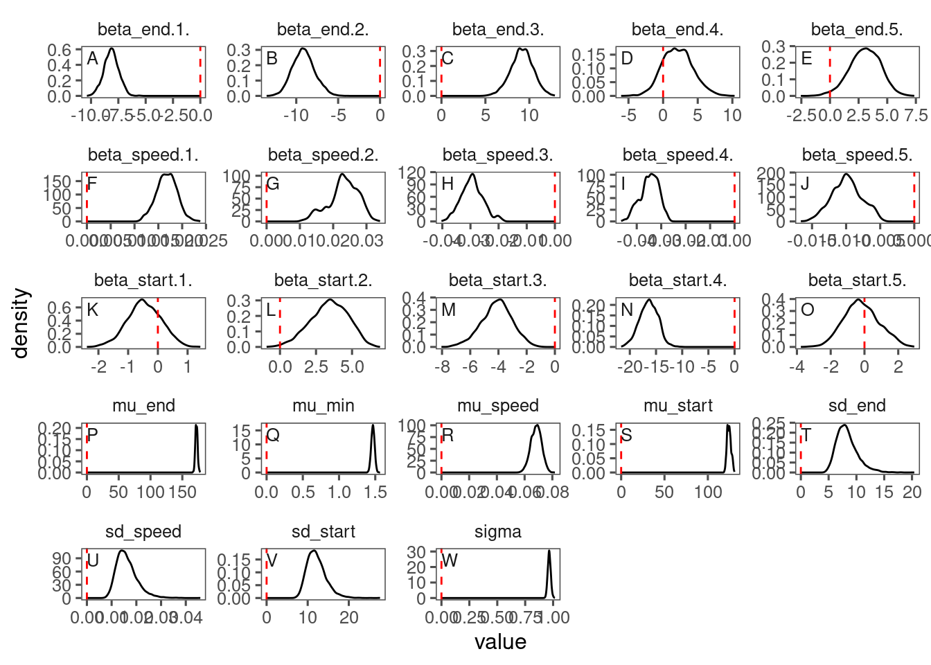
The reparameterization compiled much slower, had worse mixing, did not improve the model fit, and the inferred parameters did not look reasonable. I decided to keep the original parameterization with asym, xmid, and logk and proceed with post-hoc analyses.
Here I show the poor mixing from the reparameterized models (15, 16, and 17).
dat_15 <- dat_all %>%
  filter(species == "queru")
df_MCMC_15 <- calc_bayes_fit(
  data = dat_15 %>% mutate(tag = "training"),
  mat_prior = mat_prior,
  version = 15, # with intuitive parameterization
  num_iterations = 50000,
  nthin = 5
)
write_rds(df_MCMC_15, "alldata/intermediate/shootmodeling/df_MCMC_15.rds")
df_MCMC_15 <- read_rds("alldata/intermediate/shootmodeling/df_MCMC_15.rds") %>% tidy_mcmc(dat_15)
p_bayes_diagnostics <- plot_bayes_diagnostics(df_MCMC = df_MCMC_15)
p_bayes_diagnostics$p_MCMC
p_bayes_diagnostics$p_posterior
p_bayes_diagnostics$p_coefficient
Improving visualization of treatment effects
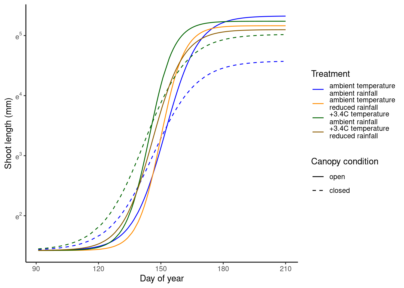
Now I make marginal predictions for each treatment combination, regardless of site and year. I hide 1.7C warming treatments and hide predictive intervals for a simpler plot. I also predict over regular grids of 91, 96, …, 210 DOYs and predicted 1,000 iterations to make the plot smoother.
df_pred_18_marginal <- calc_bayes_predict(
  data = dat_18 %>%
    distinct(heat_trt, water_trt, canopy_code, doy) %>%
    group_by(heat_trt, water_trt, canopy_code) %>%
    complete(doy = seq(91, 210, 5)) %>%
    ungroup(),
  df_MCMC = df_MCMC_18,
  version = 18,
  marginal = T,
  num_iter = 1,
  random = F
)
## [1] "1 out of 1"
p_bayes_predict_marginal <- plot_bayes_predict(
  data = dat_18,
  data_predict = df_pred_18_marginal,
  marginal = T,
  fewer_heat = T,
  vis_log = T,
  vis_ci = F
)

p_bayes_predict_marginal$p_predict
Generalize to all species
calc_bayes_all(
  data = dat_all,
  independent_priors = F, # do not use species-specific empirical informative priors
  uniform_priors = T, # use uniform priors
  intui_param = F, # regular parameterization with asym, xmid, logk
  num_iterations = 50000,
  nthin = 5,
  path = "alldata/intermediate/shootmodeling/uni/",
  num_cores = 20
)
calc_bayes_derived(path = "alldata/intermediate/shootmodeling/uni/")
plot_bayes_all(path = "alldata/intermediate/shootmodeling/uni/")
Here I only summarize the results from species with full factorial design (2 canopy conditions, 2 water treatments).
df_bayes_all <- read_bayes_all(path = "alldata/intermediate/shootmodeling/uni/", full_factorial = T, derived = T)

p_bayes_summ <- plot_bayes_summary(df_bayes_all, plot_corr = F)
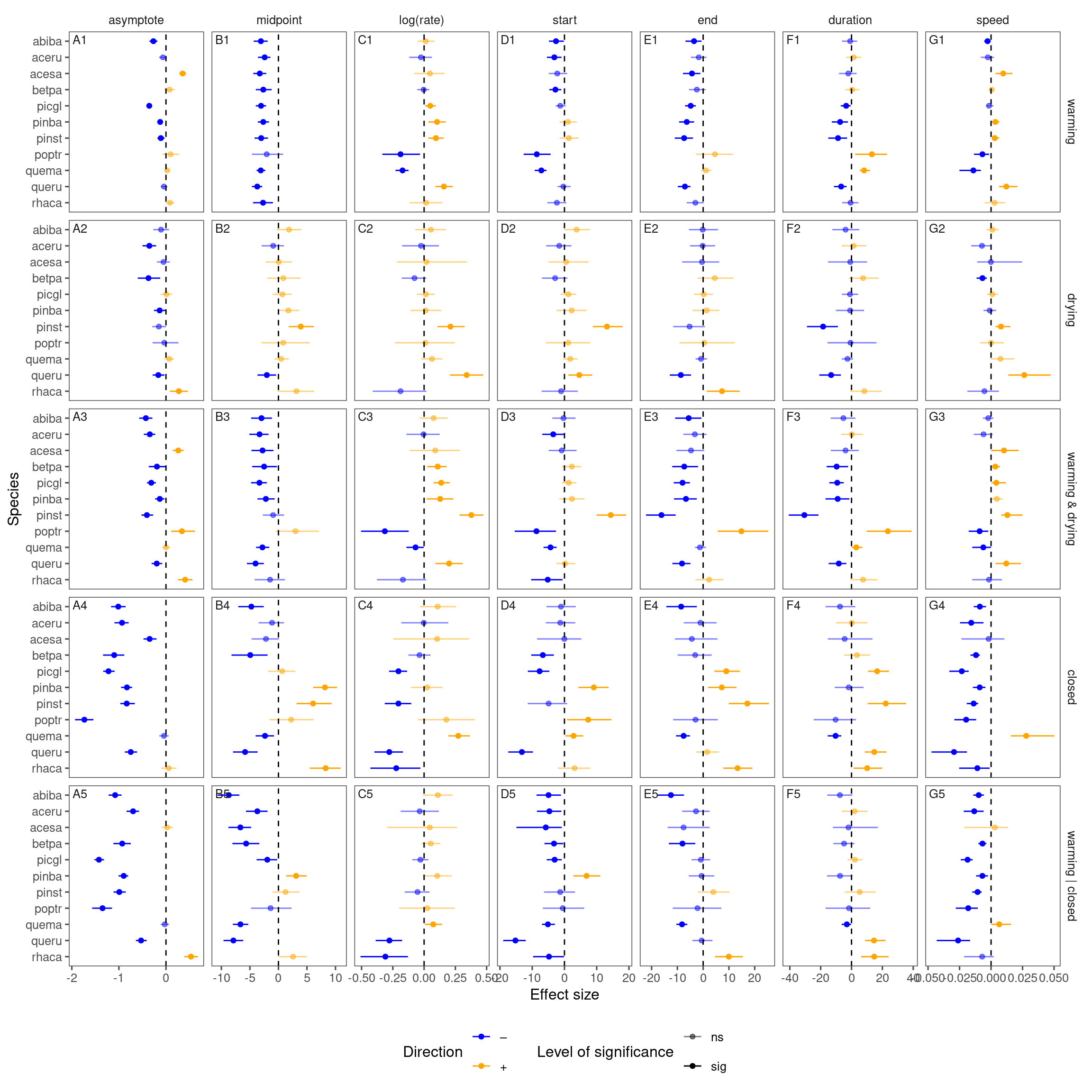
p_bayes_summ$p_coef_line
