Calculate background climatic variables using only ambient plots.

df_plot_ambient <- summ_treatment(dat_phenophase) %>%
  filter(heat_name == "ambient", water_name == "ambient") %>%
  distinct(site, canopy, block, plot)

dat_climate_spring <- summ_climate_season(dat_climate_daily, date_start = "Mar 15", date_end = "May 15", rainfall = 1)
dat_climate_spring_ambient <- dat_climate_spring %>%
  inner_join(df_plot_ambient, by = c("site", "canopy", "block", "plot")) %>%
  group_by(site, canopy, block, year) %>% # average by block
  summarise(
    temp = mean(temp),
    mois = mean(mois)
  ) %>%
  ungroup() %>%
  mutate(
    temp_std = scale(temp) %>% as.numeric(),
    mois_std = scale(mois) %>% as.numeric()
  )

dat_climate_fall <- summ_climate_season(dat_climate_daily, date_start = "Jun 15", date_end = "Sep 15", rainfall = 0)
dat_climate_fall_ambient <- dat_climate_fall %>%
  inner_join(df_plot_ambient, by = c("site", "canopy", "block", "plot")) %>%
  group_by(site, canopy, block, year) %>%
  summarise(
    temp = mean(temp),
    mois = mean(mois)
  ) %>%
  ungroup() %>%
  mutate(
    temp_std = scale(temp) %>% as.numeric(),
    mois_std = scale(mois) %>% as.numeric()
  )

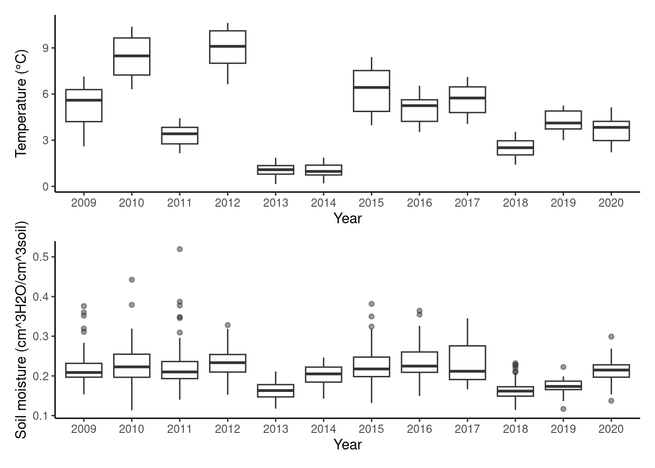
plot_climate_change(dat_climate_spring)

Calculate phenophase time and difference.

dat_phenophase_time <- dat_phenophase_time_clean %>%
  mutate(heat_trt = factor(heat_name, levels = c("ambient", "+1.7C", "+3.4C"), labels = c(0, 1, 2)) %>% as.character() %>% as.integer()) %>%
  mutate(water_trt = factor(water_name, levels = c("ambient", "reduced"), labels = c(0, 1)) %>% as.character() %>% as.integer()) %>%
  mutate(canopy_code = factor(canopy, levels = c("open", "closed"), labels = c(0, 1)) %>% as.character() %>% as.integer())

Recap of Montgomery et al. (2020)

dat_phenophase_time_summ <- summ_phenophase_time(dat_phenophase_time)
dat_phenophase_diff_summ <- calc_phenophase_diff(dat_phenophase_time_summ)

p_diff_baseline <- plot_diff_background(dat_phenophase_diff_summ, dat_climate_spring_ambient, var_x = "temp", year_range = "old", pool_sp = F)
p_diff_baseline$budbreak

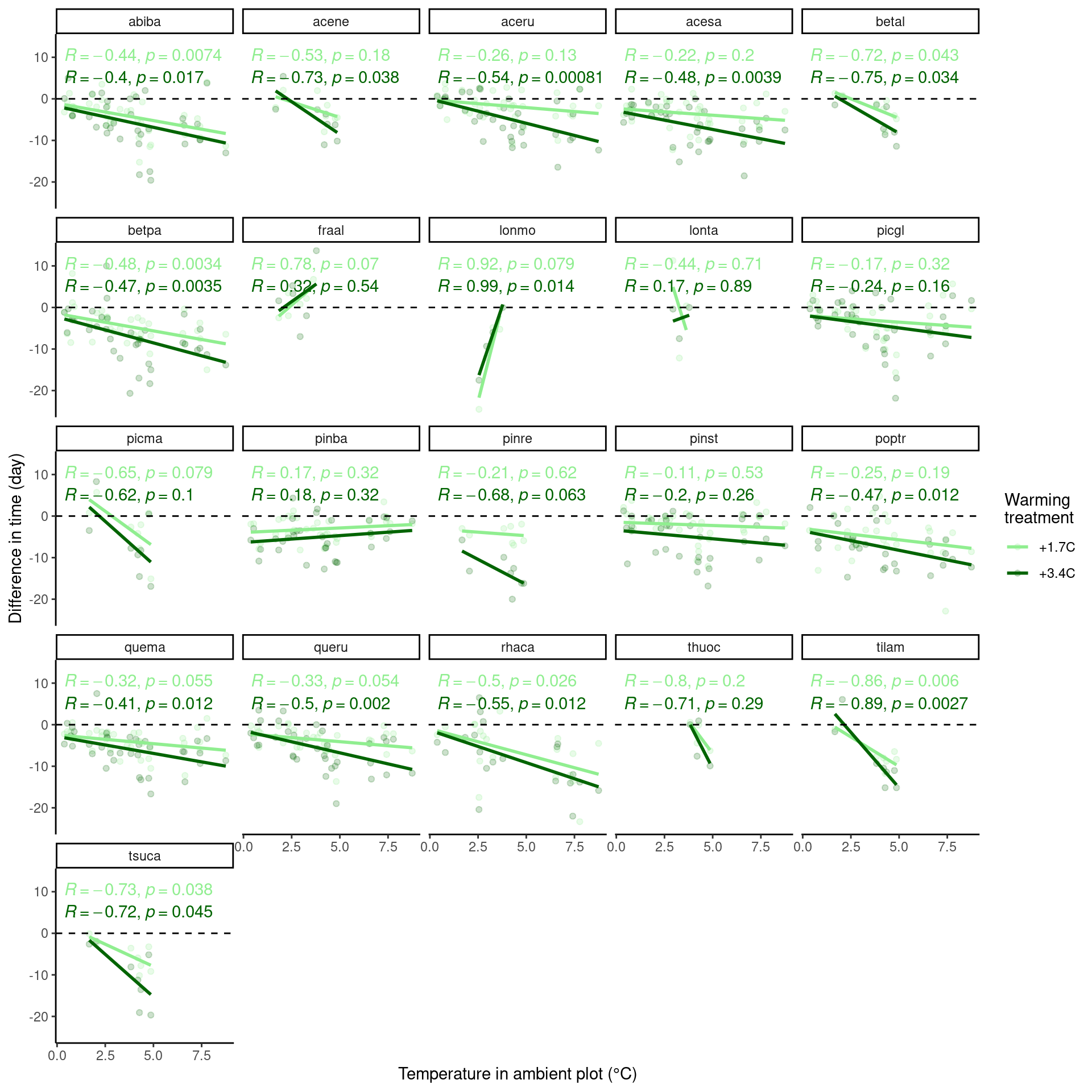
Now use data from all years.

p_diff_baseline <- plot_diff_background(dat_phenophase_diff_summ, dat_climate_spring_ambient, var_x = "temp", year_range = "full", pool_sp = F)
p_diff_baseline$budbreak

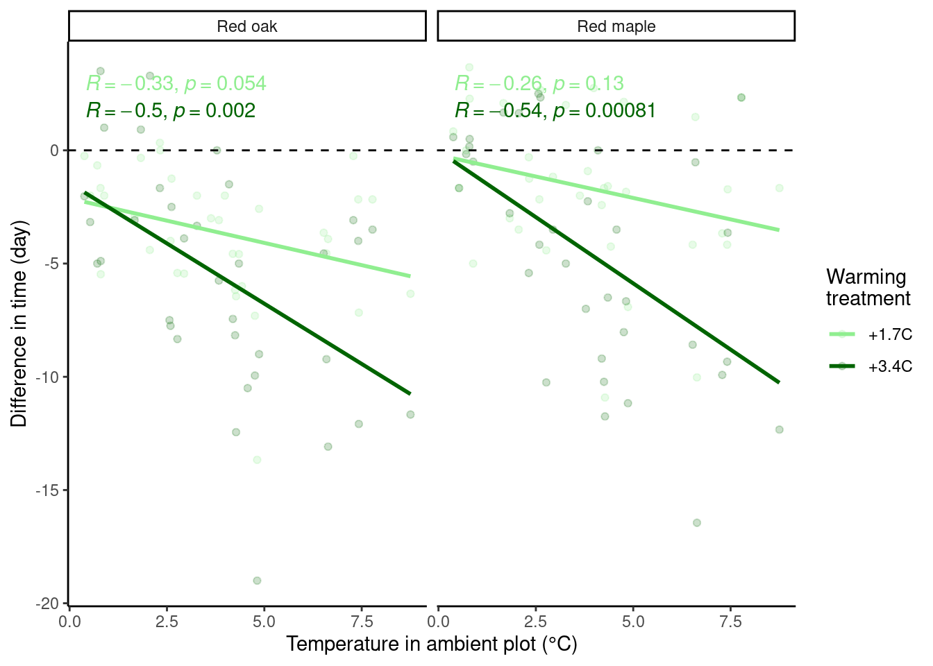
Look at two species as examples.

p_diff_baseline <- plot_diff_background(dat_phenophase_diff_summ %>%
  filter(species %in% c("queru", "aceru")) %>%
  mutate(species = factor(species,
    levels = c("queru", "aceru"),
    labels = c("Red oak", "Red maple")
  )), dat_climate_spring_ambient, var_x = "temp", year_range = "full", pool_sp = F)
p_diff_baseline$budbreak

Spring phenophases

Fit Bayesian LME for all species using package brms.

• Responses: start (budbreak), end (mostleaf), duration
• Covariates: heat, water, heat:water, canopy, heat:canopy, temp, heat:temp, mois, water:mois
• Random-effects: site-year

Join with background climate data.

dat_phenophase_time_cov <- dat_phenophase_time %>%
  left_join(dat_climate_spring_ambient, by = c("site", "canopy", "block", "year")) %>%
  group_by(species) %>%
  mutate(group = site %>% factor() %>% as.integer()) %>% # use site as random effects, not site-year
  ungroup()

test_phenophase_lme(data = dat_phenophase_time_cov, path = "alldata/intermediate/phenophase/bg/", season = "spring", chains = 1, iter = 4000, version = 3, num_cores = 5) # v3 with interactions
tidy_stanfit_all(season = "spring", path = "alldata/intermediate/phenophase/bg/")

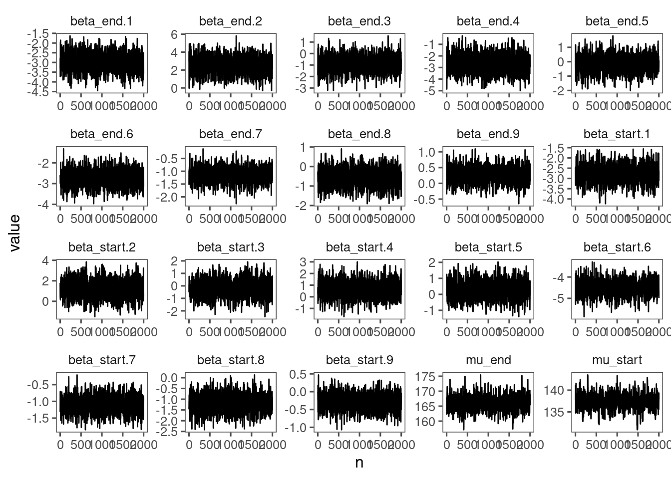
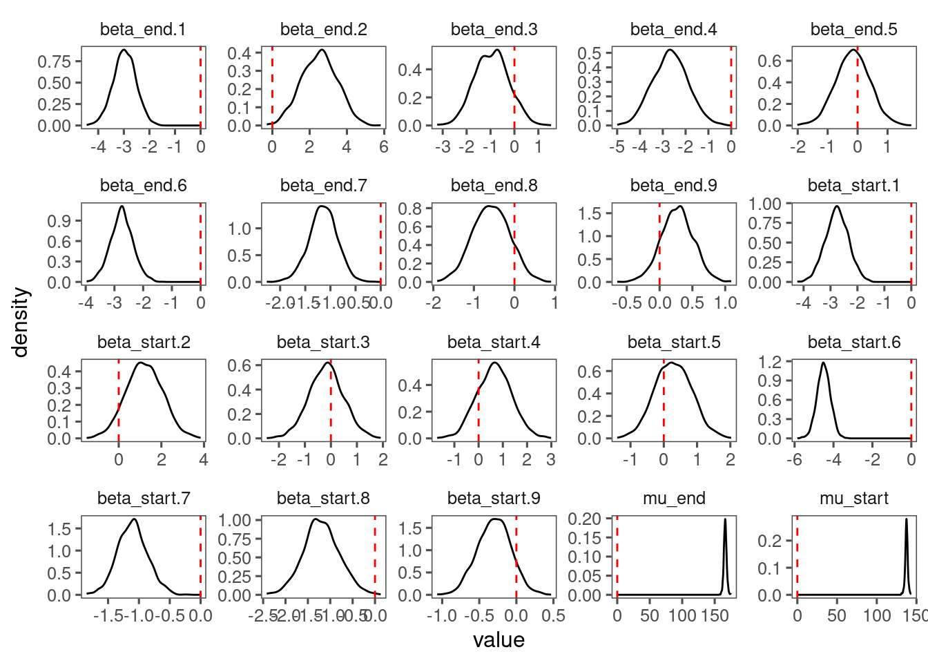
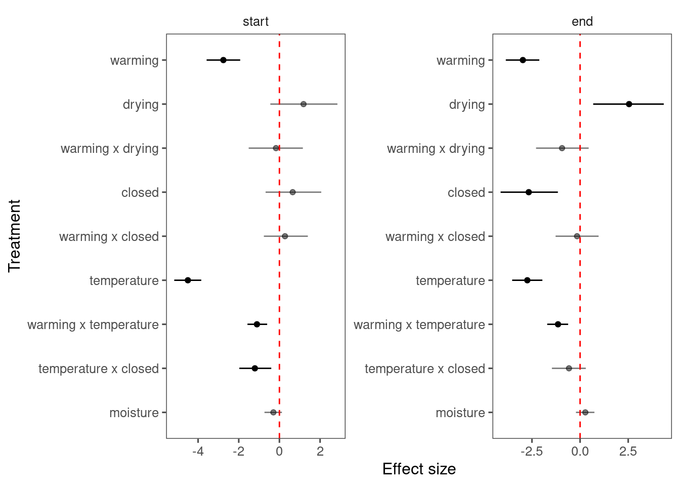
View diagnostics for spring phenology of red oak.

df_lme_all <- read_bayes_all(path = "alldata/intermediate/phenophase/bg/", season = "spring", full_factorial = T, derived = F, tidy_mcmc = F)

p_lme_diagnostics <- plot_bayes_diagnostics(df_MCMC = df_lme_all %>% filter(species == "queru"), plot_corr = F)
p_lme_diagnostics$p_MCMC

p_lme_diagnostics$p_posterior

p_lme_diagnostics$p_coefficient

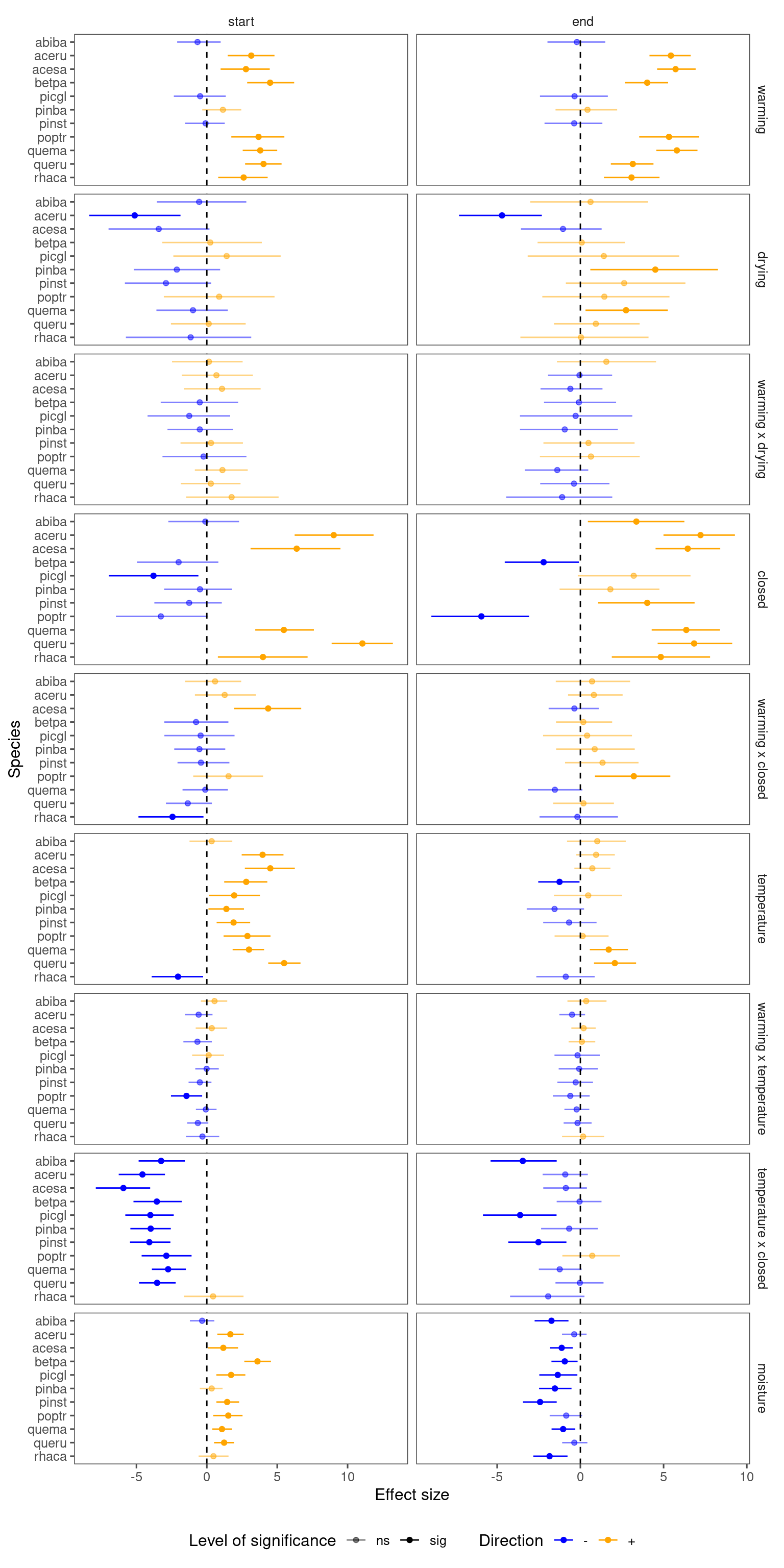
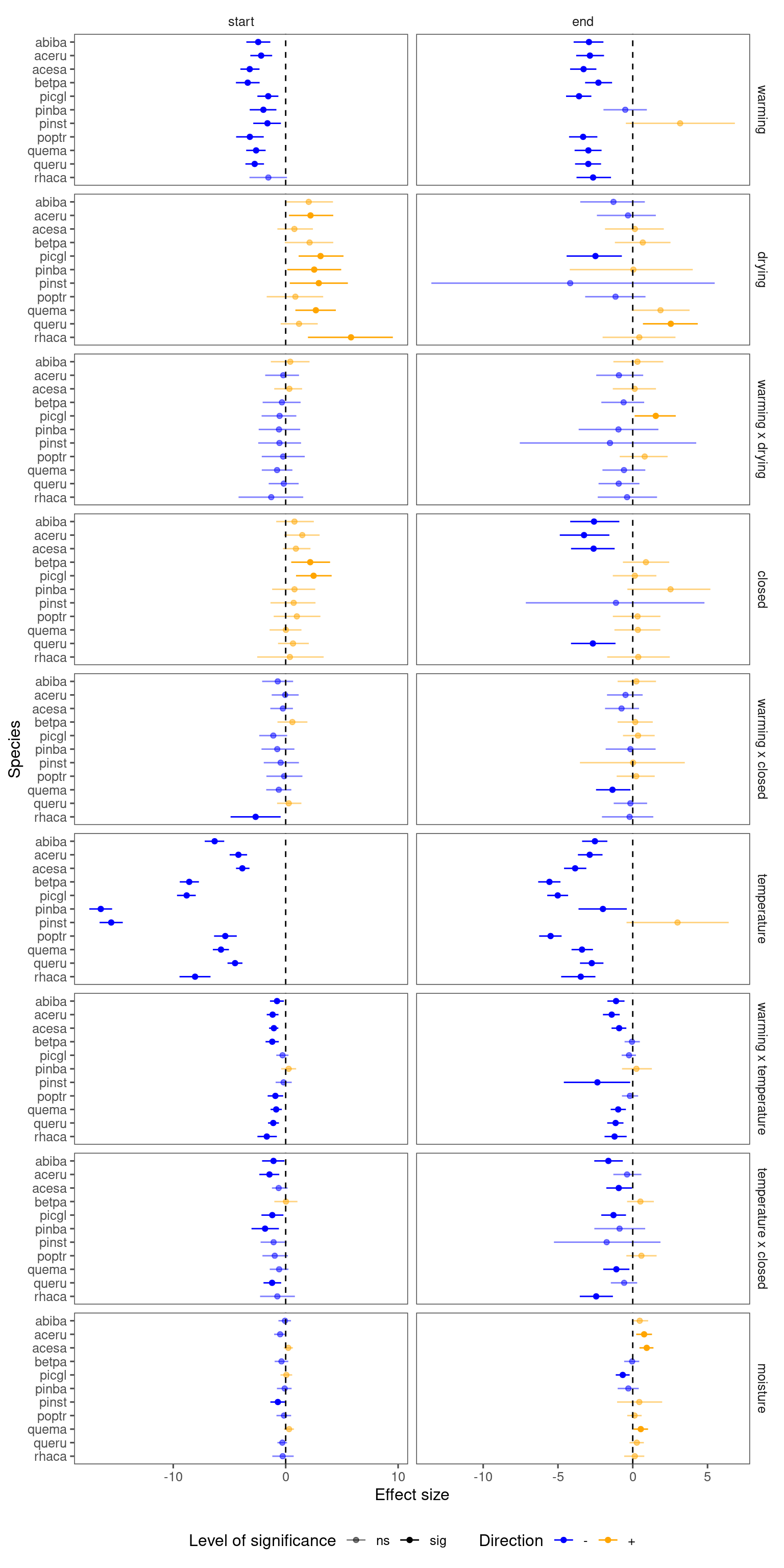
Summarize results for all species, focusing on interacting terms.

p_lme_summ <- plot_bayes_summary(
  df_lme_all,
  background = "full",
  plot_corr = F
)
p_lme_summ$p_coef_line

Fall phenophases

Fit Bayesian LME for each species using package brms.

• Responses: start (senescence), end (leafdrop), duration
• Covariates: heat, water, heat:water, canopy, heat:canopy, temp, heat:temp, mois, water:mois
• Random-effects: site-year

Join with background climate data.

dat_phenophase_time_cov <- dat_phenophase_time %>%
  left_join(dat_climate_fall_ambient, by = c("site", "canopy", "block", "year")) %>%
  group_by(species) %>%
  mutate(group = site %>% factor() %>% as.integer()) %>% # use site as random effects, not site-year
  ungroup()

test_phenophase_lme(data = dat_phenophase_time_cov, path = "alldata/intermediate/phenophase/bg/", season = "fall", chains = 1, iter = 4000, version = 3, num_cores = 5)
tidy_stanfit_all(season = "fall", path = "alldata/intermediate/phenophase/bg/")

View diagnostics for fall phenology of red oak.

df_lme_all <- read_bayes_all(path = "alldata/intermediate/phenophase/bg/", season = "fall", full_factorial = T, derived = F, tidy_mcmc = F)

p_lme_diagnostics <- plot_bayes_diagnostics(df_MCMC = df_lme_all %>% filter(species == "queru"), plot_corr = F)
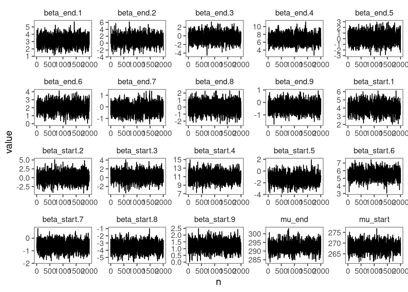
p_lme_diagnostics$p_MCMC

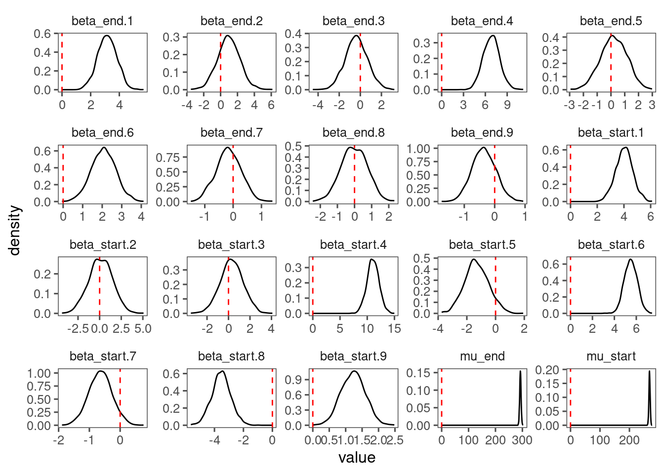
p_lme_diagnostics$p_posterior

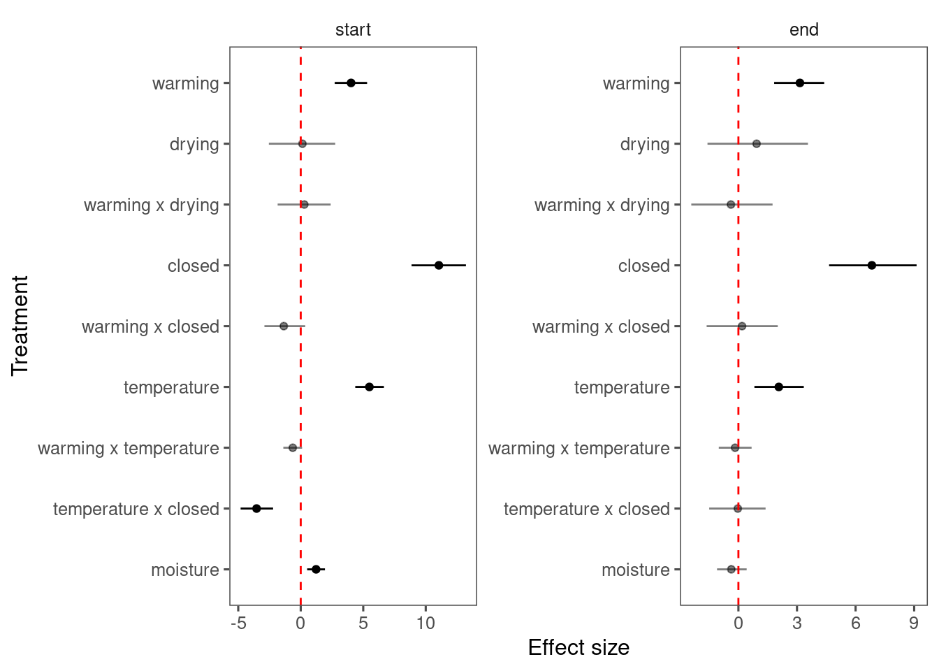
p_lme_diagnostics$p_coefficient

Summarize results for each species, focusing on interacting terms with background climate.

p_lme_summ <- plot_bayes_summary(
  df_lme_all,
  background = "full",
  plot_corr = F
)
p_lme_summ$p_coef_line