This update is focused on post-hoc analyses.

Add derived parameters

Definition

• Start: day of year reaching 5% of asymptote of logistic curve for log(shoot growth)
• End: day of year reaching 95% of asymptote of logistic curve for log(shoot growth)
• Duration: end - start, capturing the most part of shoot growth
• Speed: (95% of asymptote - 5% of asymptote) / (end - start) (reference) Note: replaced the original following definition
• Slope (at midpoint): asymptote * (1 / timescale) / 4 (reference)

Calculation

• Use posterior samples for mu and beta to recover expected parameters for each of the five treatments (except ambient).
• For interaction terms, I added up the beta for additive and interactive effects to get a total effect.
• Use mu parameters and new parameters to derive start, end, duration, and slope parameters for ambient and treatments, respectively.
• Subtract the posterior samples for derived parameters between treatment and ambient groups.
• The difference in the posteriors would be the effect size of treatments on derived parameters.
• I did something similar for random effects, but not showing the results unless we find the need to.

calc_bayes_derived(path = "alldata/intermediate/shootmodeling/all/")
plot_bayes_all(path = "alldata/intermediate/shootmodeling/all/")

Visualization

df_bayes_all_derived <- read_bayes_all(path = "alldata/intermediate/shootmodeling/all/", full_factorial = T, derived = T)
df_coef_summ <- summ_mcmc(df_bayes_all_derived)

p_bayes_summ_derived <- plot_bayes_summary(df_bayes_all_derived, plot_corr = F, subset = F)
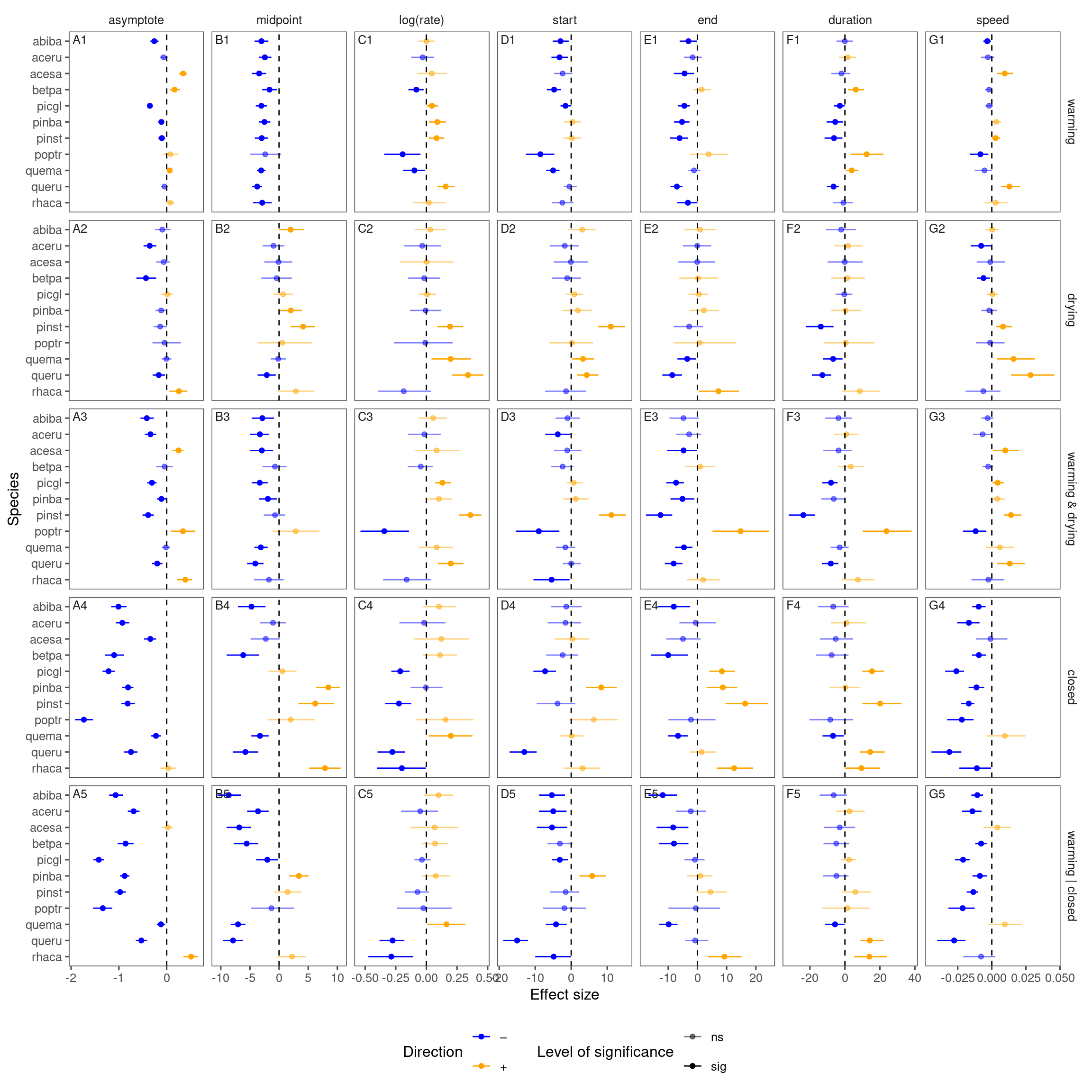
p_bayes_summ_derived$p_coef_line

Note: The coefficients for “warming x drying” and “warming x closed” now show the total effects when both treatments are present, instead of showing the interaction in addition to their additive effects.

Note: Changed parameterization to place priors on log(k) instead of the original 1/k. Calculated speed (90% asymptote / duration) to replace the original slope at inflection point for easier interpretation.

Question: The treatment effects vary by species, by there are also some consistent patterns (e.g., warming effect on midpoint). How should we summarize the results?

Decomposition of treatment effects

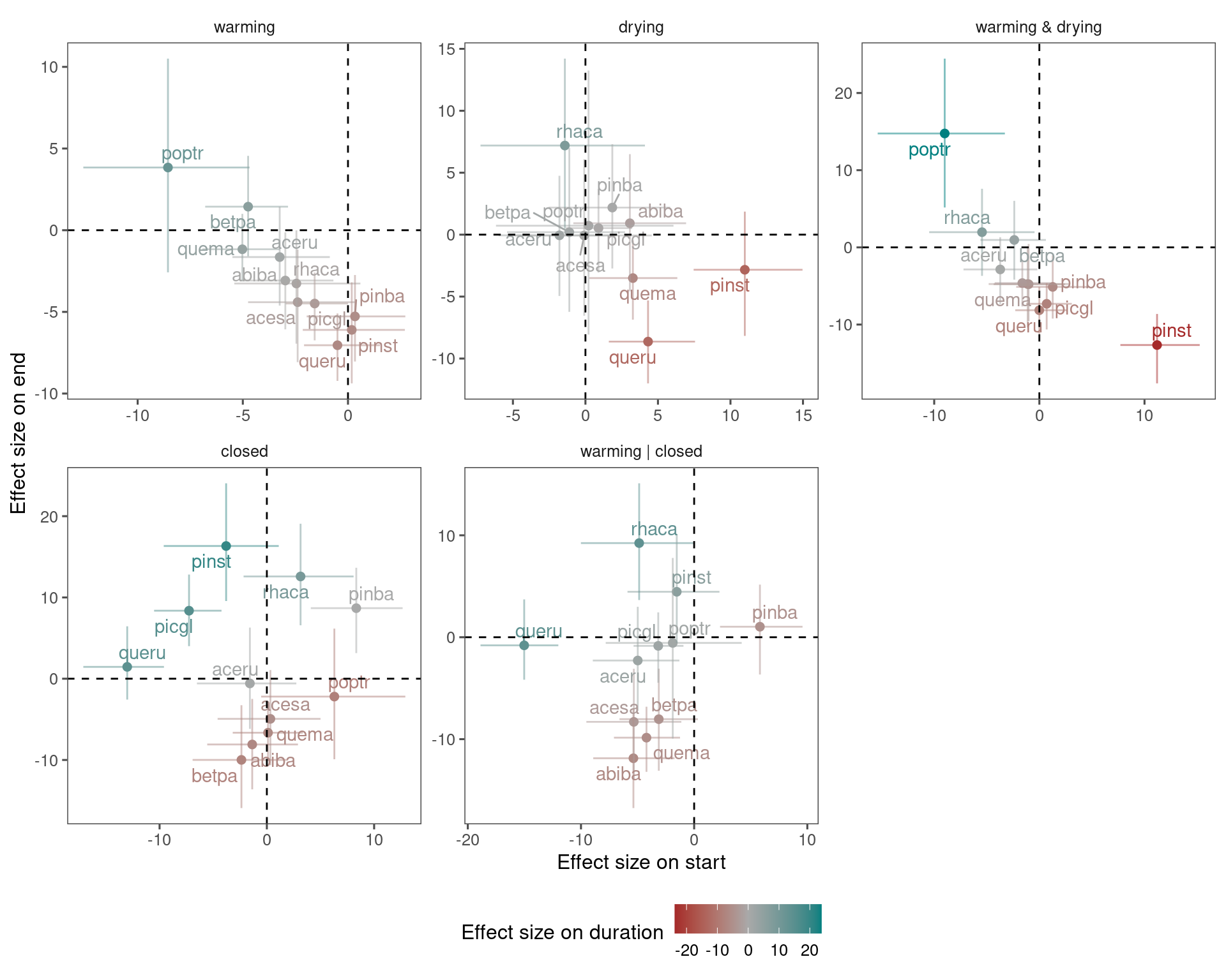
Post-hoc Question 1: Were changes in duration driven by changes in start or end?

plot_bayes_attr(df_coef_summ, var_x = "start", var_y = "end", var_col = "duration")

Interpretation: Warming induced similar advancement in both start and end, leading to little change in duration. Closed canopy induced divergent changes in duration, mainly differentiated by the response in end.

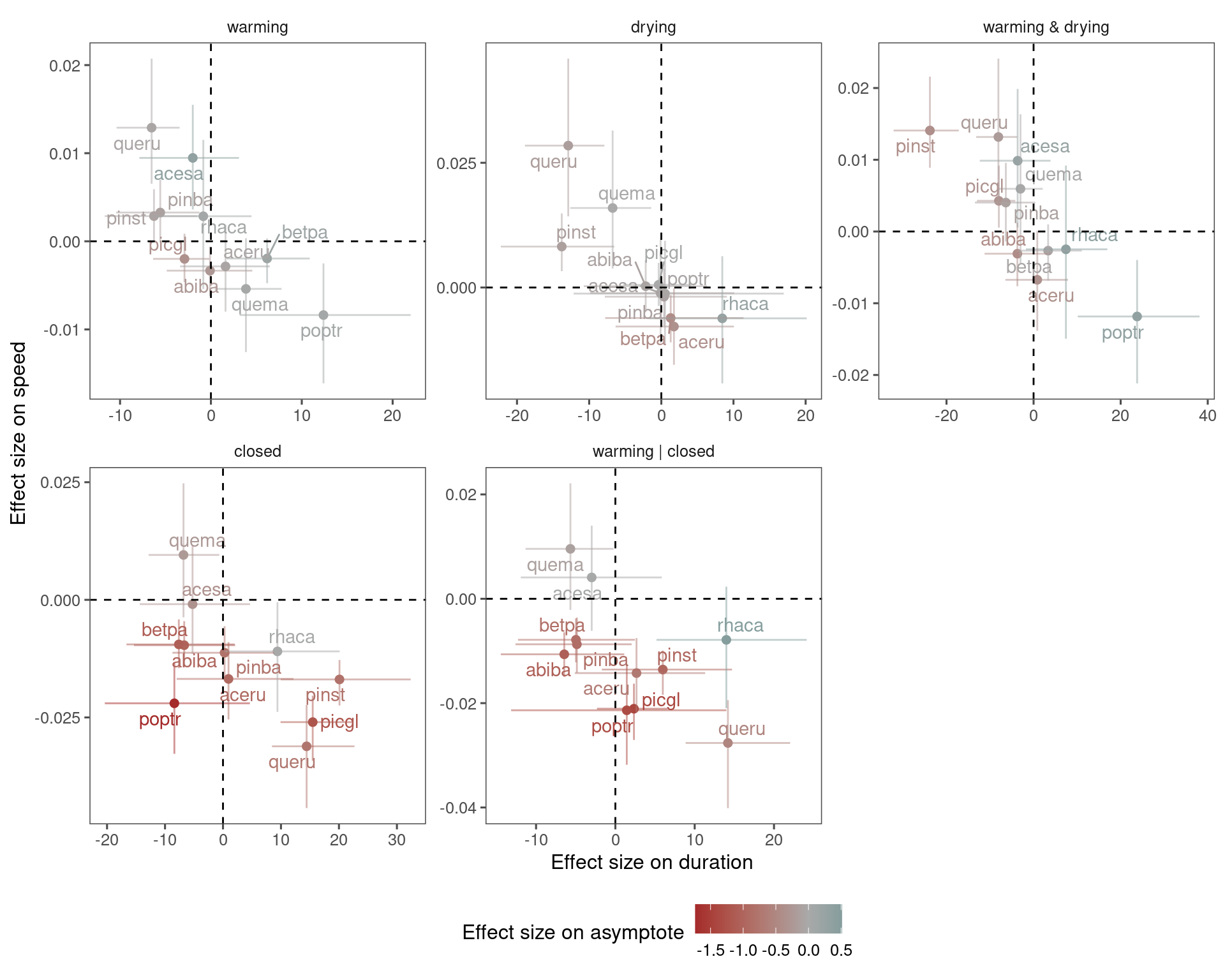
Post-hoc Question 2: Were changes in asymptote driven by changes in duration or slope?

plot_bayes_attr(df_coef_summ, var_x = "duration", var_y = "speed", var_col = "asymptote")

Interpretation: Lower asymptotes from closed canopy were driven by a combination of shorter duration and slower speed. There seems to be a trade-off between an increase in duration and an increase in speed under warming and drying, but the overall changes in asymptote were small.