Bayesian model 9

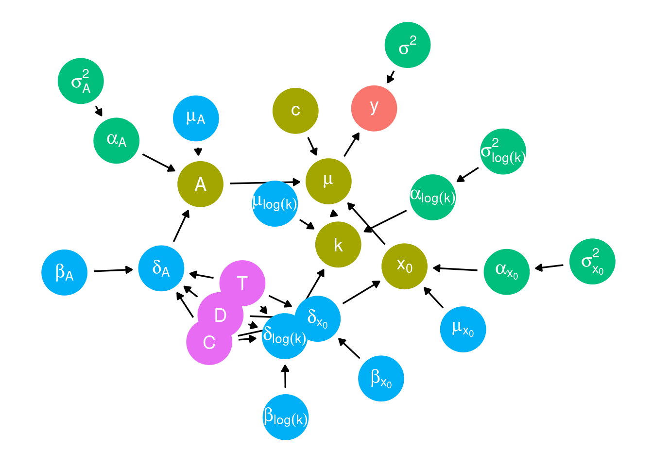
Based on Model 6. Site-year-level random effects. Ignore block-level, plot-level, individual-level differences. Treatments as covariates. Canopy as an additive term and interaction term with warming treatment.

Model

Data model

\begin{align*} y_{i,t,s,d} \sim \text{Lognormal}(\mu_{i,t,s,d}, \sigma^2) \end{align*}

Process model

\begin{align*} \mu_{i,t,s,d} &= c+\frac{A_{i,t,s}}{1+e^{-k_{i,t,s}(d-x_{0 i,t,s})}} \newline A_{i,t,s} &= \mu_A + \delta_{A,i}+ \alpha_{A,t,s} \newline x_{0 i,t,s} &= \mu_{x_0} + \delta_{x_0,i}+ \alpha_{x_0,t,s} \newline log(k_{i,t,s}) &= \mu_{log(k)} + \delta_{log(k),i}+ \alpha_{log(k),t,s} \end{align*}

Fixed effects

\begin{align*} \delta_{A,i} &= \beta_{A,1} T_i + \beta_{A,2} D_i + \beta_{A,3} T_i D_i + \beta_{A,4} C_i + \beta_{A,5} T_i C_i \newline \delta_{x_0,i} &= \beta_{x_0,1} T_i + \beta_{x_0,2} D_i + \beta_{x_0,3} T_i D_i + \beta_{x_0,4} C_i + \beta_{x_0,5} T_i C_i \newline \delta_{log(k),i} &= \beta_{log(k),1} T_i + \beta_{log(k),2} D_i + \beta_{log(k),3} T_i D_i + \beta_{log(k),4} C_i + \beta_{log(k),5} T_i C_i \end{align*}

Random effects

\begin{align*} \alpha_{A,t,s} &\sim \text{Normal}(0, \sigma_A^2) \newline \alpha_{x_0,t,s} &\sim \text{Normal}(0, \sigma_{x_0}^2) \newline \alpha_{log(k),t,s} &\sim \text{Normal}(0, \sigma_{log(k)}^2) \end{align*}

Priors

\begin{align*} c &\sim \text{Normal}(0, 1) \newline \mu_A &\sim \text{Normal}(5, 1) \newline \beta_A &\sim \text{Multivariate Normal} ( \begin{pmatrix} 0 \newline 0 \newline 0 \newline 0 \newline 0 \newline \end{pmatrix}, \begin{pmatrix} 1 & 0 & 0 & 0 & 0 \newline 0 & 1 & 0 & 0 & 0 \newline 0 & 0 & 1 & 0 & 0 \newline 0 & 0 & 0 & 1 & 0 \newline 0 & 0 & 0 & 0 & 1 \newline \end{pmatrix} )\newline \sigma_A^2 &\sim \text{Truncated Normal}(0, 1, 0, \infty) \newline \mu_{x_0} &\sim \text{Normal}(160, 100) \newline \beta_{x_0} &\sim \text{Multivariate Normal} ( \begin{pmatrix} 0 \newline 0 \newline 0 \newline 0 \newline 0 \newline \end{pmatrix}, \begin{pmatrix} 100 & 0 & 0 & 0 & 0 \newline 0 & 100 & 0 & 0 & 0 \newline 0 & 0 & 100 & 0 & 0 \newline 0 & 0 & 0 & 100 & 0 \newline 0 & 0 & 0 & 0 & 100 \newline \end{pmatrix} )\newline \sigma_{x_0}^2 &\sim \text{Truncated Normal}(0, 100, 0, \infty) \newline \mu_{log(k)} &\sim \text{Normal}(-2, 0.04, 0, \infty) \newline \beta_{log(k)} &\sim \text{Multivariate Normal} ( \begin{pmatrix} 0 \newline 0 \newline 0 \newline 0 \newline 0 \newline \end{pmatrix}, \begin{pmatrix} 0.04 & 0 & 0 & 0 & 0 \newline 0 & 0.04 & 0 & 0 & 0 \newline 0 & 0 & 0.04 & 0 & 0 \newline 0 & 0 & 0 & 0.04 & 0 \newline 0 & 0 & 0 & 0 & 0.04 \newline \end{pmatrix} )\newline \sigma_{log(k)}^2 &\sim \text{Truncated Normal}(0, 0.04, 0, \infty) \newline \sigma^2 &\sim \text{Truncated Normal}(0, 1, 0, \infty) \end{align*}

Draw a DAG.

plot_bayes_dag(version = 9)

Prepare data

dat_9 <- dat_shoot_cov %>%
  filter(species == "queru") %>%
  filter(doy > 90, doy <= 210) %>%
  filter(shoot > 0) %>%
  drop_na(barcode) %>%
  mutate(group = str_c(site, year, sep = "_") %>% factor() %>% as.integer()) %>%
  mutate(heat_trt = factor(heat_name, levels = c("ambient", "+1.7C", "+3.4C"), labels = c(0, 1, 2)) %>% as.character() %>% as.integer()) %>%
  mutate(water_trt = factor(water_name, levels = c("ambient", "reduced"), labels = c(0, 1)) %>% as.character() %>% as.integer()) %>%
  mutate(canopy_code = factor(canopy, levels = c("open", "closed"), labels = c(0, 1)) %>% as.character() %>% as.integer())

Note that I selected for data between day 91 (Apr) and day 210 (Jul).

Fit model

df_MCMC_9 <- calc_bayes_fit(
  data = dat_9 %>% mutate(tag = "training"),
  version = 9,
  num_iterations = 50000,
  nthin = 5
)
write_rds(df_MCMC_9, "alldata/intermediate/shootmodeling/df_MCMC_9.rds")

df_MCMC_9 <- read_rds("alldata/intermediate/shootmodeling/df_MCMC_9.rds") %>%
  tidy_mcmc(dat_9)
p_bayes_diagnostics <- plot_bayes_diagnostics(df_MCMC = df_MCMC_9)
p_bayes_diagnostics$p_MCMC

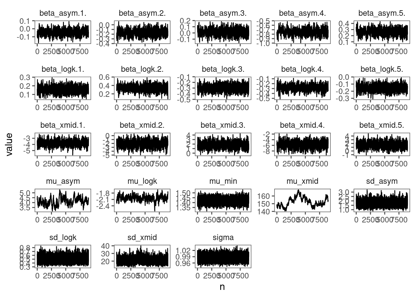Speed is acceptable (~ 20 min). Mixing is ok. Using a longer chain (50,000 instead of 10,000 and thinned by a factor of 5).

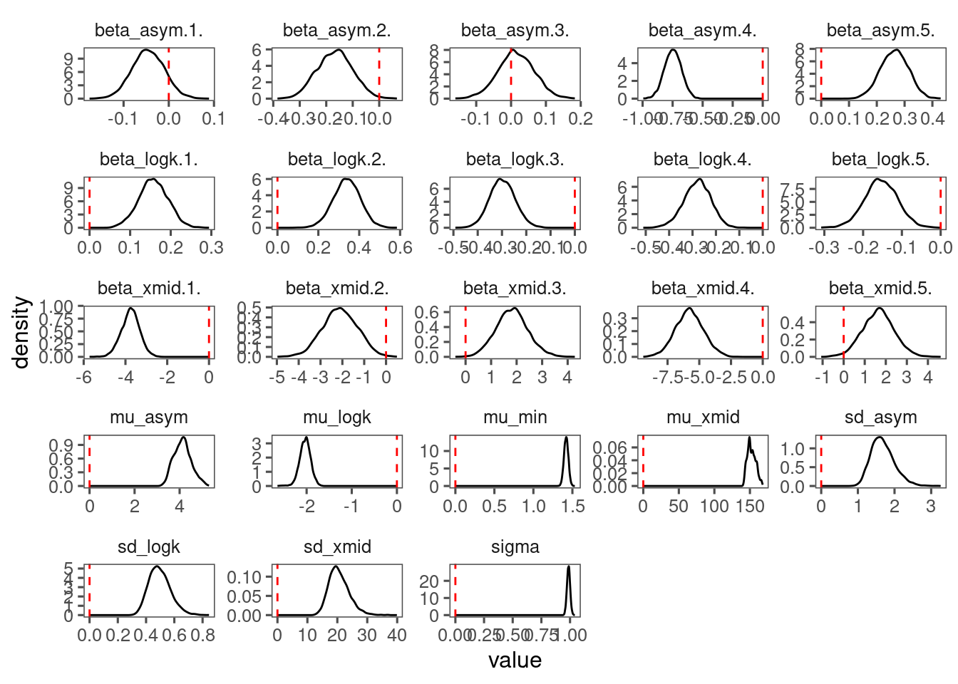
p_bayes_diagnostics$p_posterior

p_bayes_diagnostics$p_coefficient

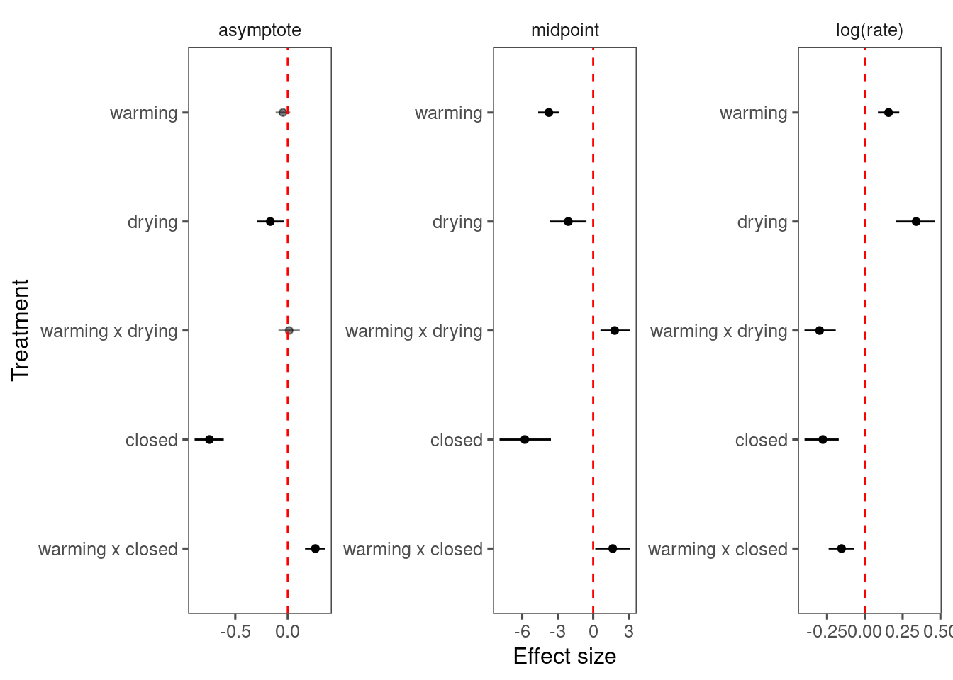
Inference:

Drying and closed canopy reduce asymptote.
Warming increases asymptote under closed canopy.
Warming, drying, closed canopy advance midpoint.
The advancing effect of warming is attenuated by drying and closed canopy condition.
No significant effect on growth time

p_bayes_diagnostics$p_correlation

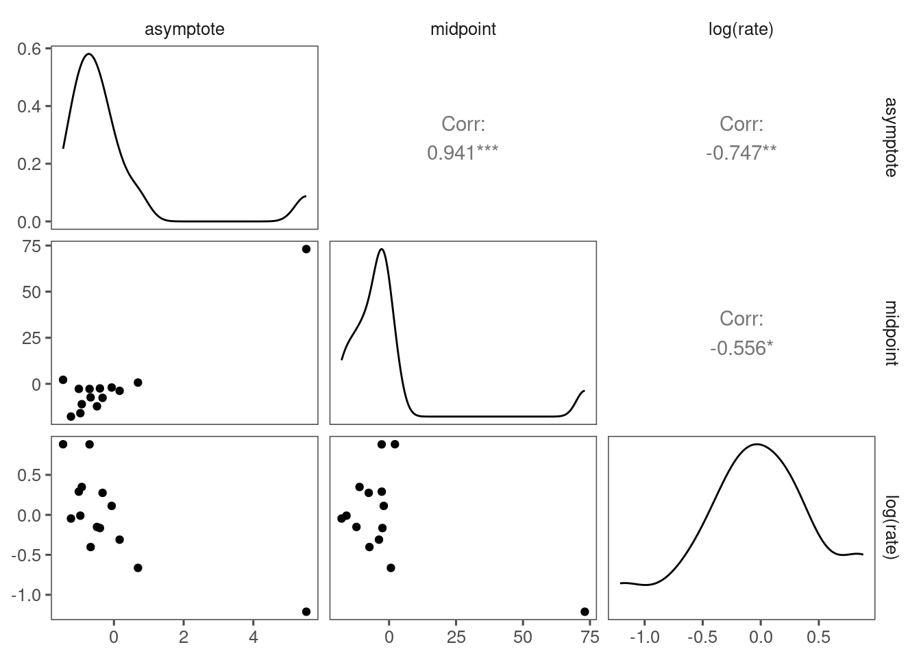Did not see significant correlation among inferred random effects.

Make predictions

df_pred_9 <- calc_bayes_predict(
  data = dat_9 %>%
    distinct(site, year, group, heat_trt, water_trt, canopy, canopy_code, doy),
  df_MCMC = df_MCMC_9,
  version = 9
)
write_rds(df_pred_9, "alldata/intermediate/shootmodeling/df_pred_9.rds")

df_pred_9 <- read_rds("alldata/intermediate/shootmodeling/df_pred_9.rds")
p_bayes_predict <- plot_bayes_predict(
  data = dat_9,
  data_predict = df_pred_9,
  vis_log = T
)

p_bayes_predict$p_original

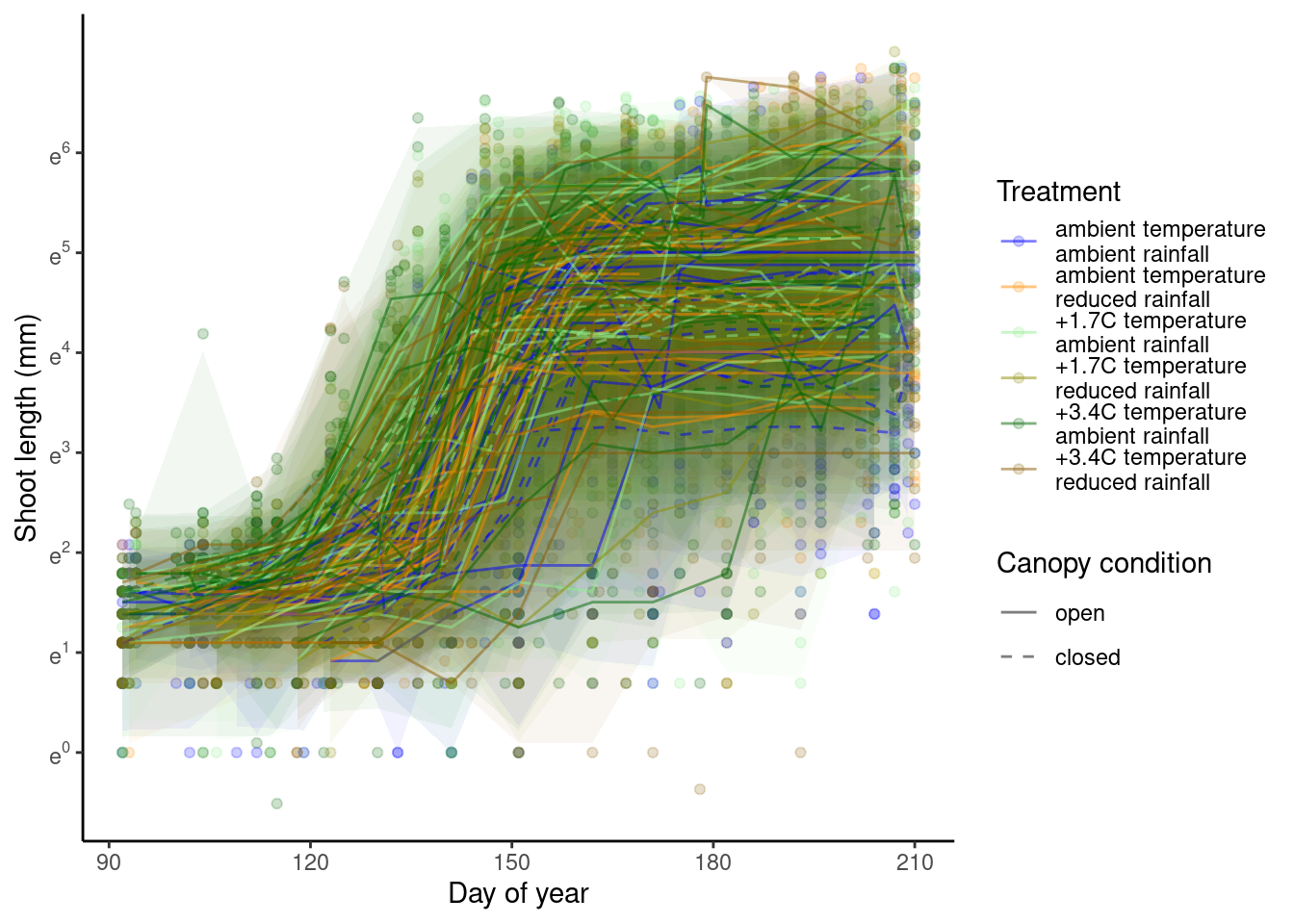
p_bayes_predict$p_overlay

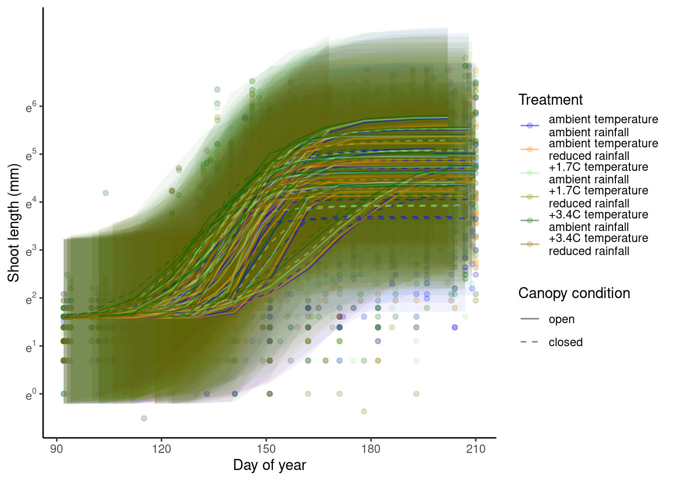
p_bayes_predict$p_accuracy

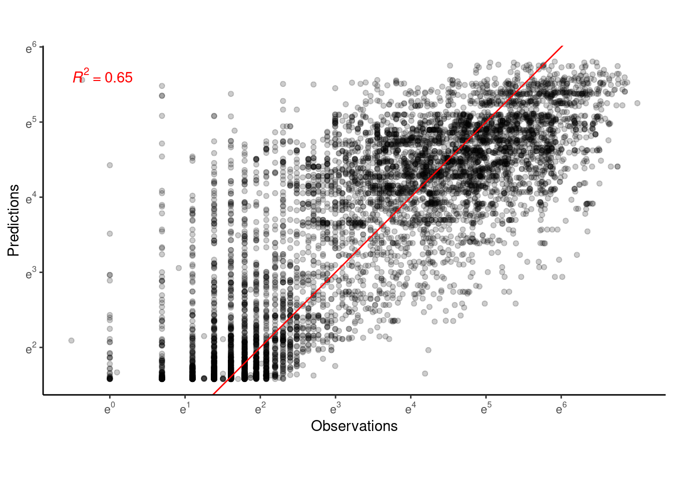
Visualize year 2016 and site HWRC alone.

p_bayes_predict <- plot_bayes_predict(
  data = dat_9 %>% filter(year == 2016, site == "hwrc"),
  data_predict = df_pred_9 %>% filter(year == 2016, site == "hwrc"),
  vis_log = T
)
p_bayes_predict$p_original

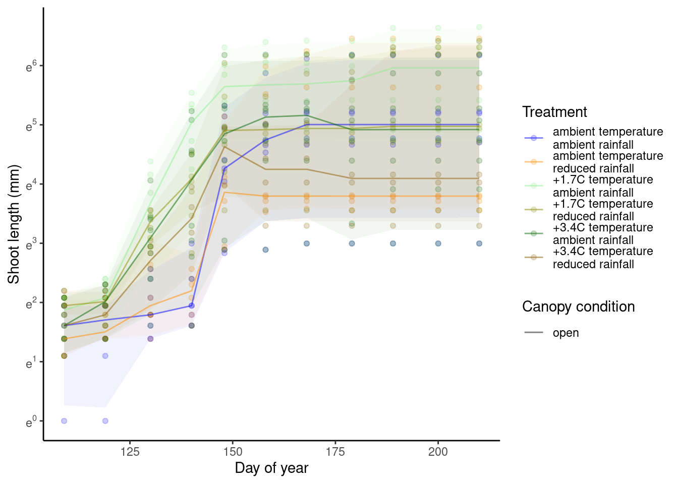
p_bayes_predict$p_overlay

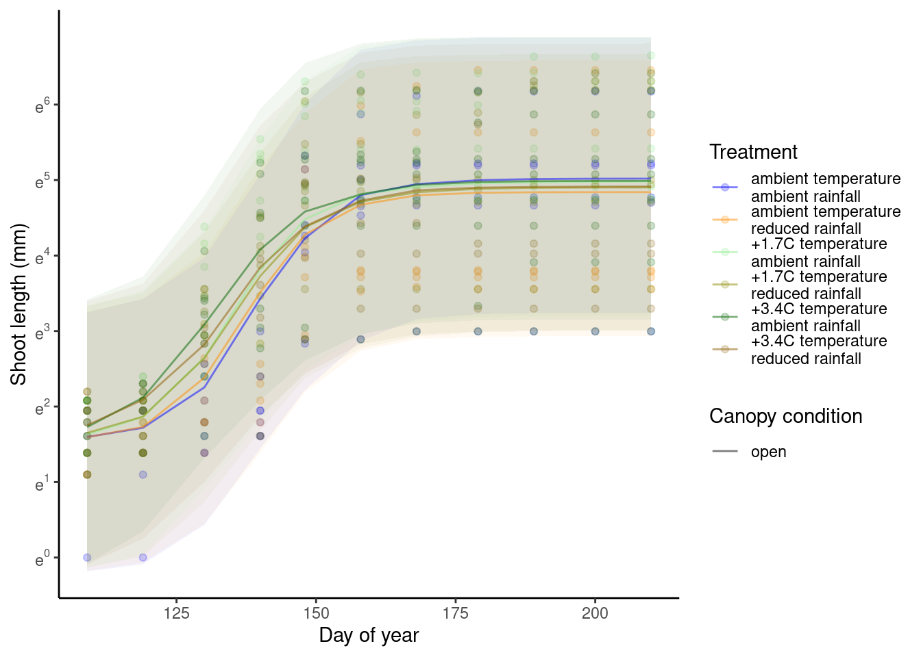
Generalize to all species

Fit a separate model for each species.

Adjustments in models:

For species with both canopy conditions and both water treatments, use Model 9.
For species with one canopy condition and both water treatments, use Model 10.
For species with one canopy condition and one water treatment, use Model 11.

dat_all <- dat_shoot_cov %>%
  filter(doy > 90, doy <= 210) %>%
  filter(shoot > 0) %>%
  drop_na(barcode) %>%
  group_by(species) %>%
  mutate(group = str_c(site, year, sep = "_") %>% factor() %>% as.integer()) %>%
  ungroup() %>%
  mutate(heat_trt = factor(heat_name, levels = c("ambient", "+1.7C", "+3.4C"), labels = c(0, 1, 2)) %>% as.character() %>% as.integer()) %>%
  mutate(water_trt = factor(water_name, levels = c("ambient", "reduced"), labels = c(0, 1)) %>% as.character() %>% as.integer()) %>%
  mutate(canopy_code = factor(canopy, levels = c("open", "closed"), labels = c(0, 1)) %>% as.character() %>% as.integer())

calc_bayes_all(
  data = dat_all,
  num_iterations = 50000,
  nthin = 5,
  path = "alldata/intermediate/shootmodeling/all/",
  num_cores = 20
)
plot_bayes_all(path = "alldata/intermediate/shootmodeling/all/")

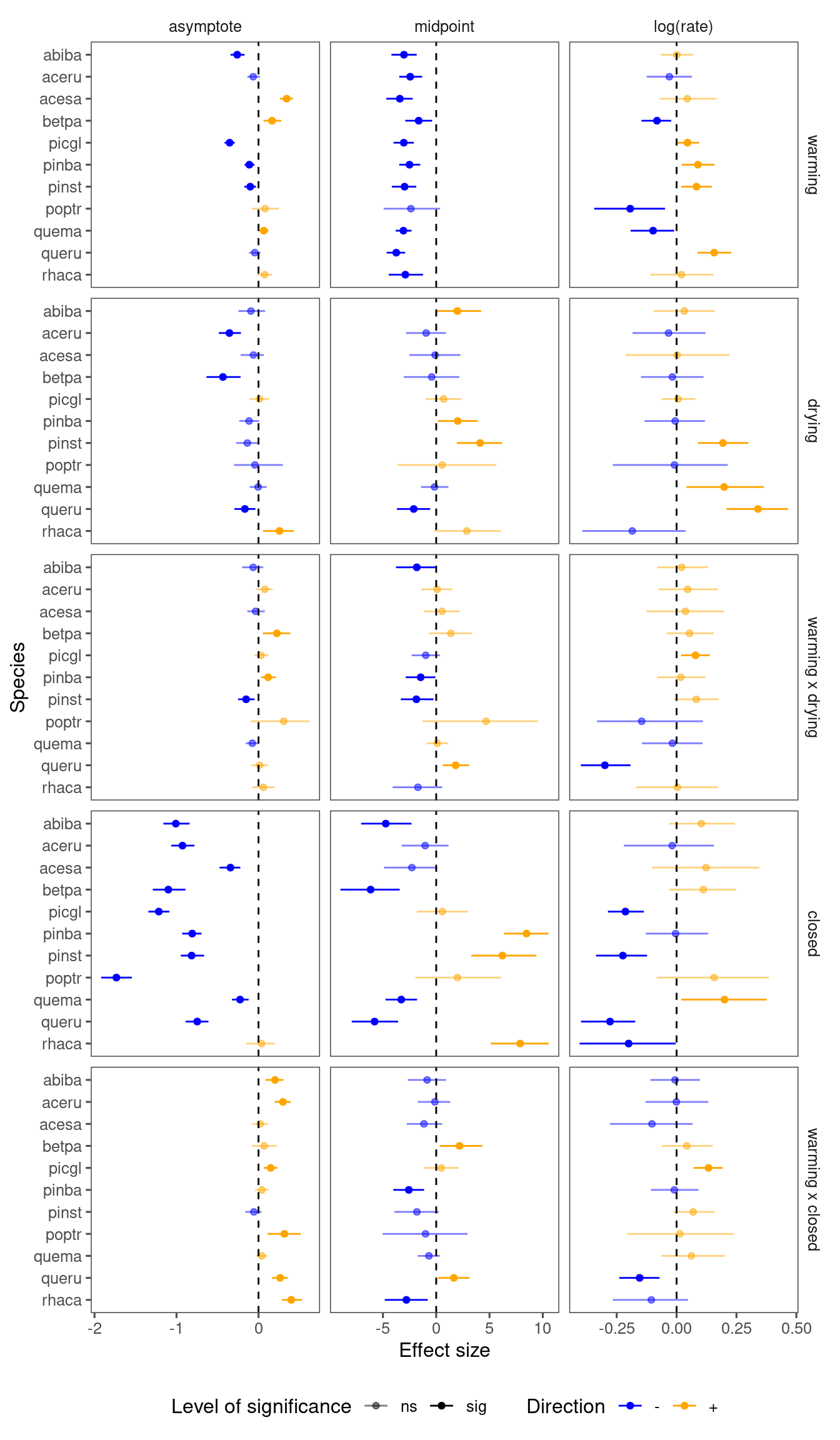
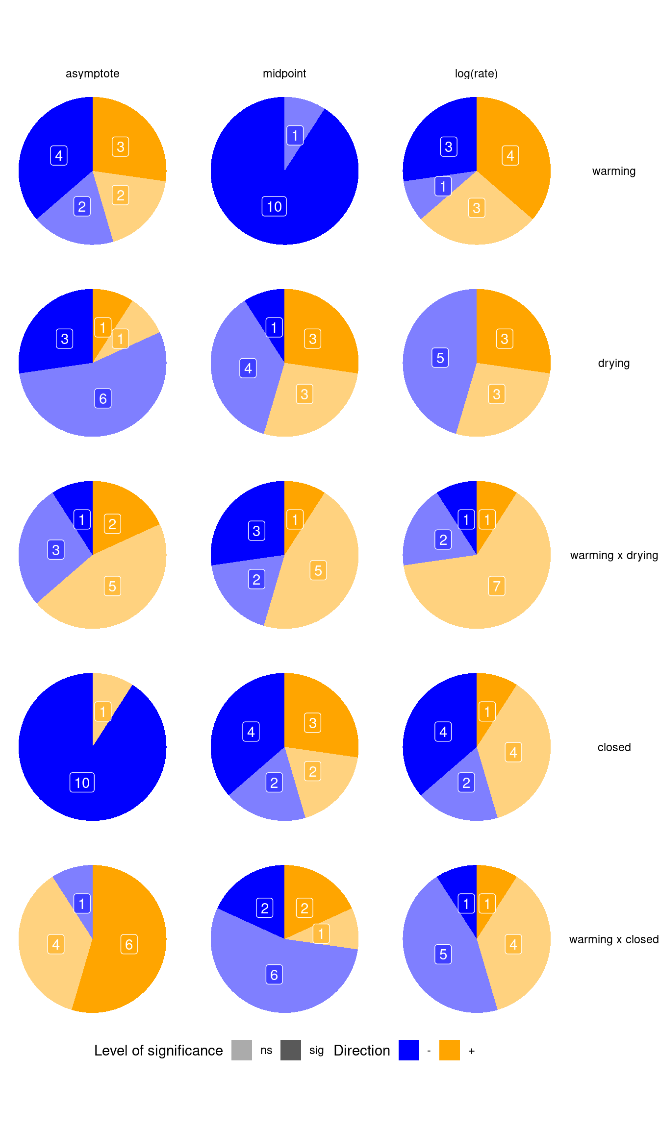
Here I only summarize the results from species with full factorial design (2 canopy conditions, 2 water treatments).

df_bayes_all <- read_bayes_all(path = "alldata/intermediate/shootmodeling/all/", full_factorial = T)
df_coef_summ <- summ_mcmc(df_bayes_all)
df_coef_summ %>%
  arrange(response, covariate, desc(median)) %>%
  select(response, covariate, category, median, lower, upper, species) %>%
  group_by(response, covariate, category) %>%
  summarise(species = toString(species), .groups = "drop")

## # A tibble: 54 × 4
##    response  covariate        category                   species                
##    <fct>     <fct>            <fct>                      <chr>                  
##  1 asymptote warming          positive (significant)     acesa, betpa, quema    
##  2 asymptote warming          positive (non-significant) poptr, rhaca           
##  3 asymptote warming          negative (non-significant) queru, aceru           
##  4 asymptote warming          negative (significant)     pinst, pinba, abiba, p…
##  5 asymptote drying           positive (significant)     rhaca                  
##  6 asymptote drying           positive (non-significant) picgl                  
##  7 asymptote drying           negative (non-significant) quema, poptr, acesa, a…
##  8 asymptote drying           negative (significant)     queru, aceru, betpa    
##  9 asymptote warming x drying positive (significant)     betpa, pinba           
## 10 asymptote warming x drying positive (non-significant) poptr, aceru, rhaca, p…
## # ℹ 44 more rows

p_bayes_summ <- plot_bayes_summary(df_bayes_all)
p_bayes_summ$p_coef_line

p_bayes_summ$p_coef_pie

p_bayes_summ$p_coef_pca

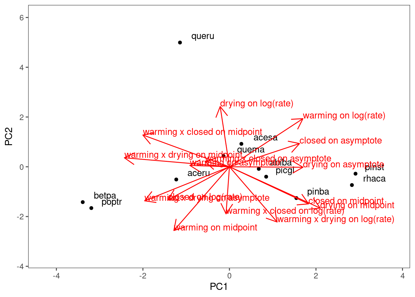
Climate change effects (summarizing the majority):

Warming advances midpoint.
Drying reduces asymptote, delays midpoint.
Under drying, the effect of warming is more likely to further increase asymptote.
Closed canopy reduces asymptote.
Under closed canopy, the effect of warming is more likely to increase asymptote.

p_bayes_summ$p_corr_pie

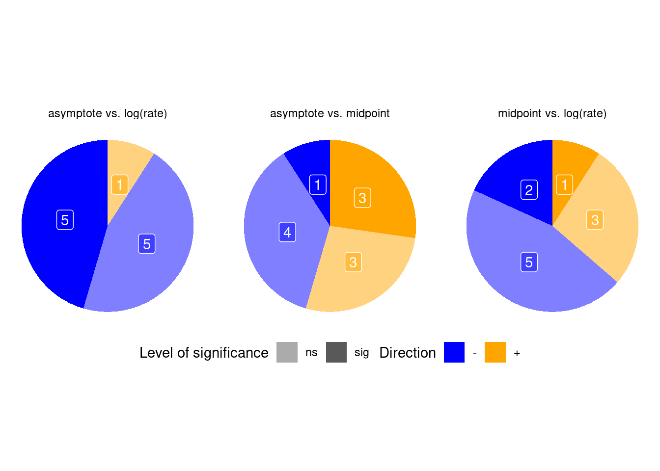
Correlation between parameters (summarizing the majority):