Tidy shoot growth data
dat_shoot <- tidy_shoot()

usethis::proj_set(str_c(getwd(), "/phenologyb4warmed/"), force = T)
setwd("phenologyb4warmed/")
usethis::use_data(dat_shoot, overwrite = T)
setwd("..")
Shoot length data saved in package. Use directly.
Questions about data: * Some plants have barcode of NA. Removed. * Some plants have multiple slots. Separating the slots in groups. * One shoot length record was 6806. Removed shoot length greater than 5000. * I’m guessing the unit of shoot length is mm.
dat_shoot %>% head(10)## # A tibble: 10 × 15
## site canopy heat heat_name water water_name block plot species barcode
## <chr> <fct> <fct> <fct> <fct> <fct> <chr> <chr> <chr> <dbl>
## 1 cfc open _ ambient _ ambient d d4 abiba 365
## 2 cfc open _ ambient _ ambient d d4 abiba 365
## 3 cfc open _ ambient _ ambient d d4 abiba 365
## 4 cfc open _ ambient _ ambient d d4 abiba 365
## 5 cfc open _ ambient _ ambient d d4 abiba 365
## 6 cfc open _ ambient _ ambient d d4 abiba 365
## 7 cfc open _ ambient _ ambient d d4 abiba 365
## 8 cfc open _ ambient _ ambient d d4 abiba 365
## 9 cfc open _ ambient _ ambient d d4 abiba 365
## 10 cfc open _ ambient _ ambient d d4 abiba 365
## # ℹ 5 more variables: cohort <dbl>, slot <chr>, year <dbl>, doy <dbl>,
## # shoot <dbl>Exploratory plots
plot_shoot_sampling(dat_shoot)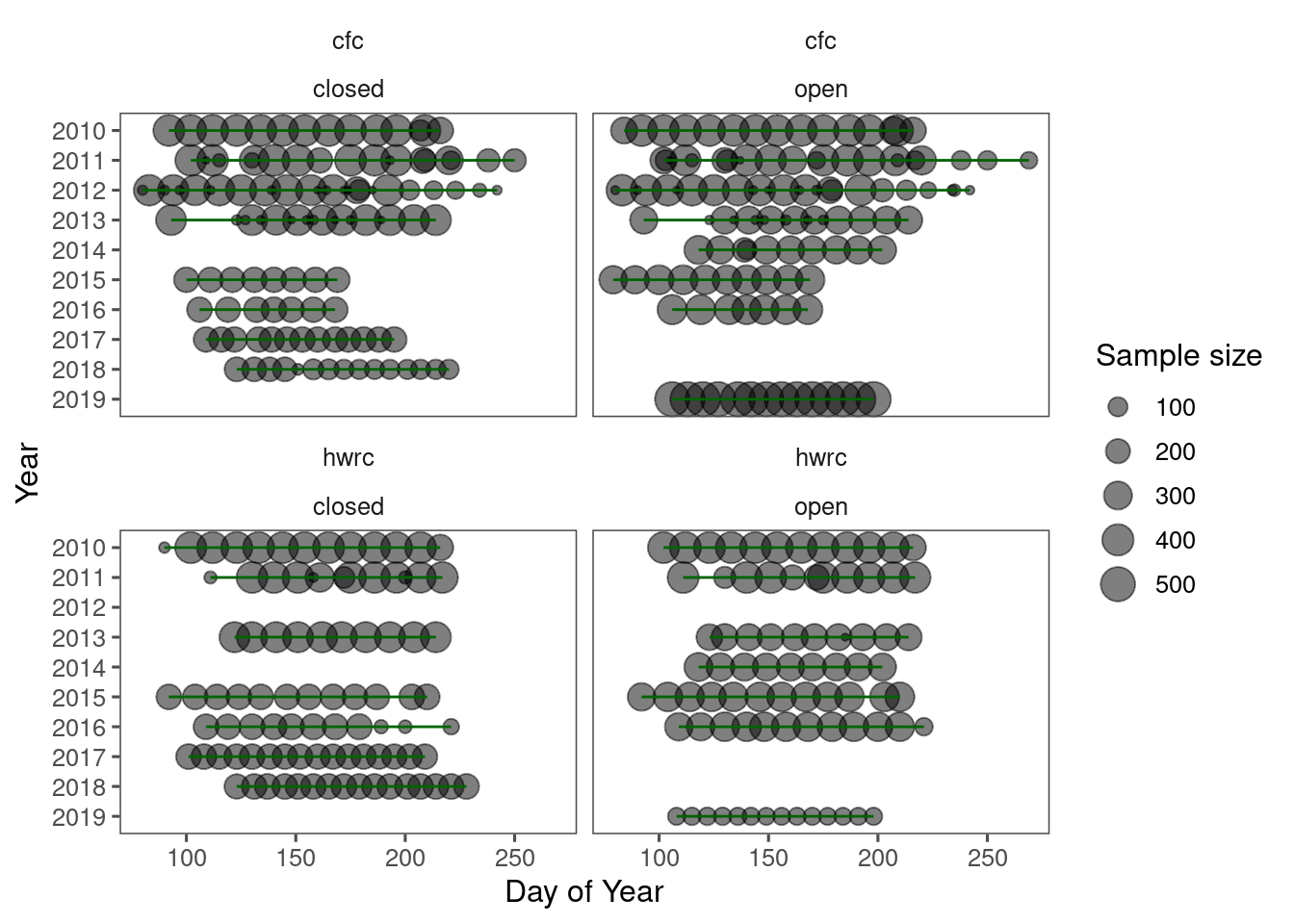
Questions about sampling methods: * How were the sampling periods determined? * How were the sampling frequencies or intervals determined?
plot_shoot(dat_shoot %>% filter(species == "queru"))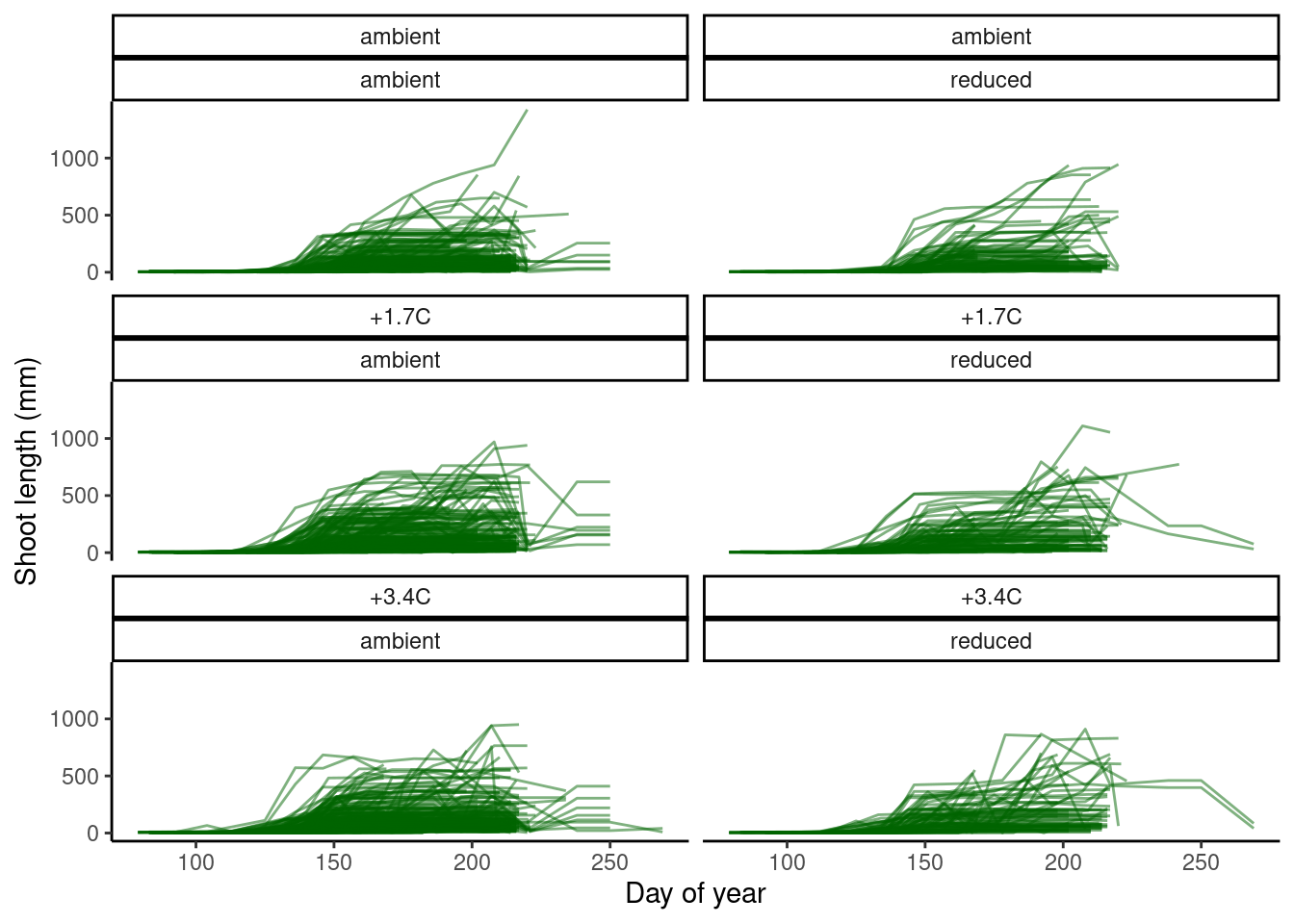
plot_shoot(dat_shoot %>% filter(species == "queru"), quantile = T)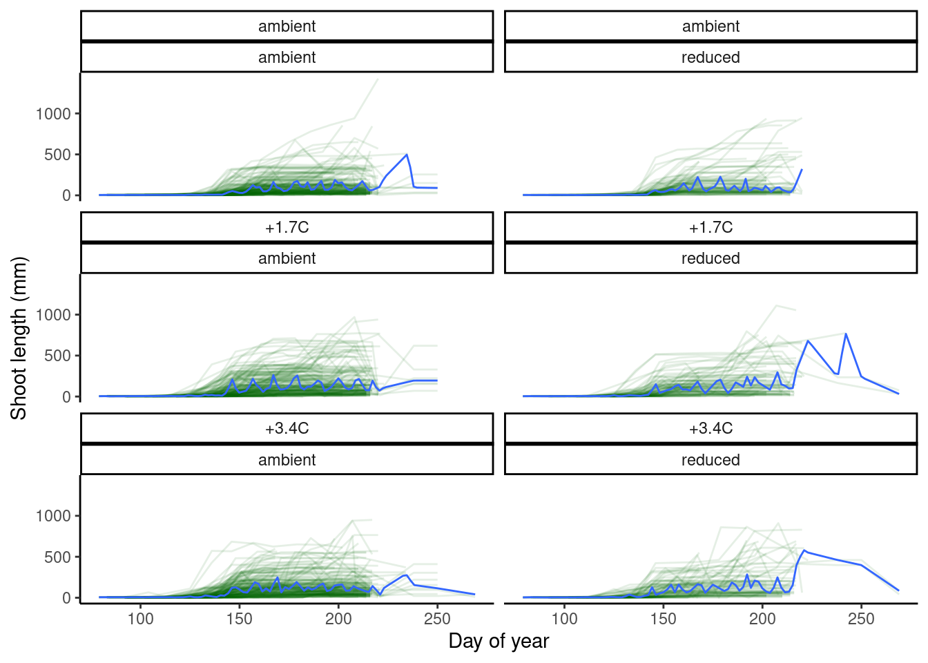
Quantile regression
Using specific sites, canopy conditions, species as examples.
test_shoot_quantreg(dat_shoot %>%
  filter(species == "queru", canopy == "open", site == "cfc") %>%
  filter(doy >= 120, doy < 170)) %>%
  summary()
## Call:
## quantregGrowth::gcrq(formula = shoot ~ ps(doy, monotone = 1) +
## heat + water + heat_water, tau = 0.5, data = df)
##
## -------- Percentile: 0.50 check function: 36588 -----
##
## parametric terms:
## Est StErr |z| p-value
## (Intercept) 49.350 3.106 15.89 < 2e-16 ***
## heat 5.344 1.893 2.82 0.00476 **
## water 1.743 2.805 0.62 0.53429
## heat_water -3.131 2.618 1.20 0.23175
## ---
## Signif. codes: 0 '***' 0.001 '**' 0.01 '*' 0.05 '.' 0.1 ' ' 1
##
## smooth terms:
## edf
## ps(doy) 5.997
## =========================
##
## No. of obs = 1368 No. of params = 15 (15 for each quantile)
## Overall check = 36588.42 SIC = 3.313 on edf = 10 (ncross constr: FALSE)test_shoot_quantreg(dat_shoot %>%
filter(species == "aceru", canopy == "open", site == "cfc") %>%
filter(doy >= 120, doy < 170)) %>%
summary()## Call:
## quantregGrowth::gcrq(formula = shoot ~ ps(doy, monotone = 1) +
## heat + water + heat_water, tau = 0.5, data = df)
##
## -------- Percentile: 0.50 check function: 20657 -----
##
## parametric terms:
## Est StErr |z| p-value
## (Intercept) 37.1097 2.1114 17.58 < 2e-16 ***
## heat 2.9007 0.9726 2.98 0.00286 **
## water 0.4003 1.5658 0.26 0.79823
## heat_water -1.4996 1.3408 1.12 0.26339
## ---
## Signif. codes: 0 '***' 0.001 '**' 0.01 '*' 0.05 '.' 0.1 ' ' 1
##
## smooth terms:
## edf
## ps(doy) 4
## =========================
##
## No. of obs = 1365 No. of params = 15 (15 for each quantile)
## Overall check = 20656.62 SIC = 2.738 on edf = 8 (ncross constr: FALSE)- Warming tends to promote shoot growth.
- Rainfall reduction effect also tends to promote shoot growth (not conclusive).
- Interaction between warming and drying might offset promoted shoot growth.
- Note that random effects not implemented.
- Reminder than this is a very rough descriptive analysis with no parametric models or random effects.
Five growth models
dat_growth_model <- calc_compare_growth_model(dat_shoot %>% filter(species == "queru", canopy == "open", site == "cfc"))
plot_compare_growth_model(dat_growth_model, option = "fit")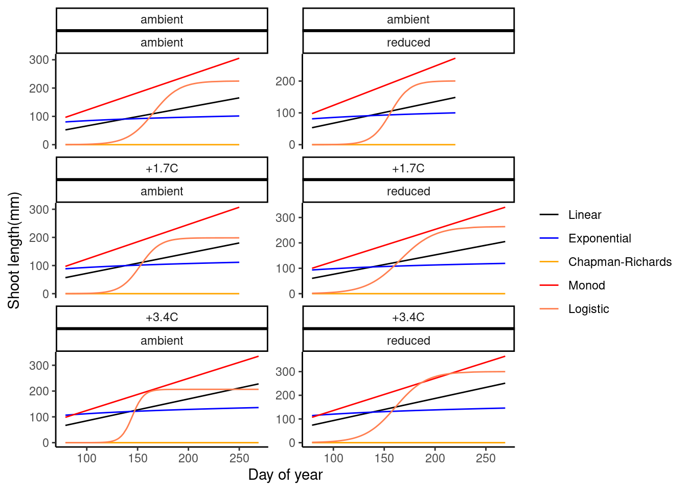
plot_compare_growth_model(dat_growth_model, option = "test")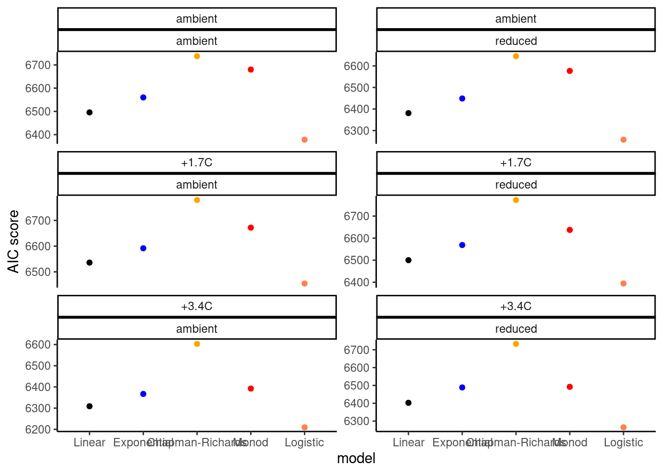
dat_growth_model <- calc_compare_growth_model(dat_shoot %>% filter(species == "aceru", canopy == "open", site == "cfc"))
plot_compare_growth_model(dat_growth_model, option = "fit")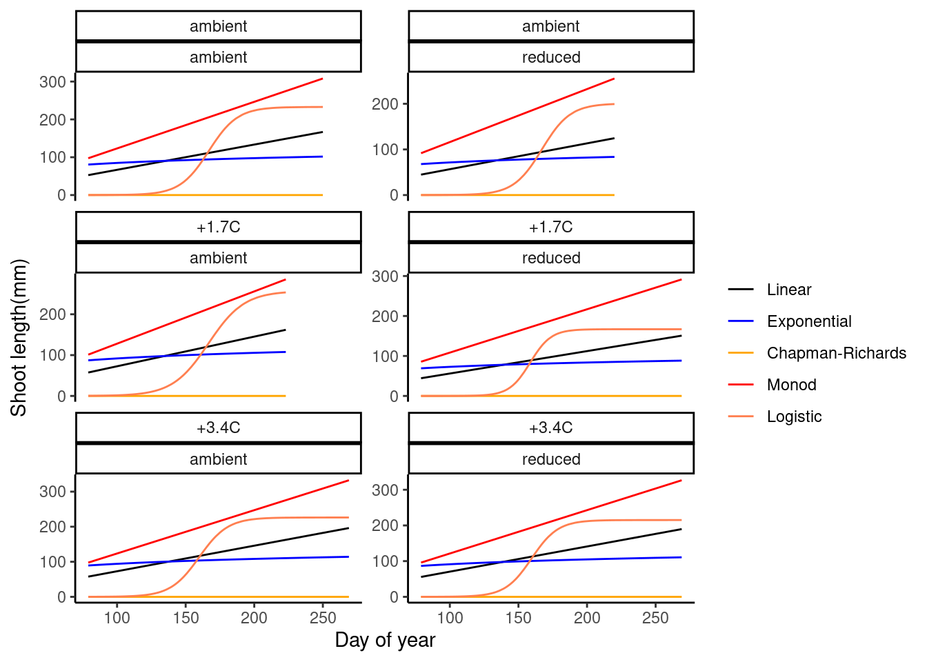
plot_compare_growth_model(dat_growth_model, option = "test")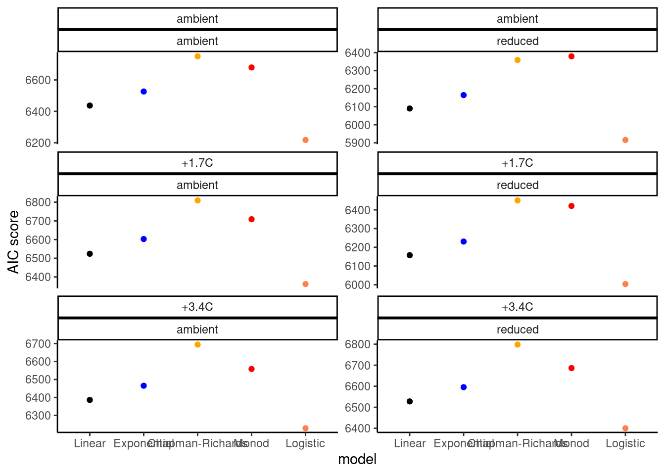
- Logistic model seems to be reasonable.
- Exponential, Chapman-Richards, and Monod models have fast increases at the start, which don’t work well with data during dormancy.
- Additional parameter to control the starting time of rapid increase?
Bayesian model
Prepare data for model fitting.
dat <- dat_shoot %>%
  filter(species == "queru", canopy == "open", site == "cfc") %>%
  filter(shoot > 0)
Fit a most basic lognormal logistic function with a subset of data. No covariates. No random effects.
df_MCMC <- calc_bayes_fit(
  data = dat %>% mutate(tag = "training"),
  version = 1
)
## ===== Monitors =====
## thin = 1: asym, logk, min, sigma, xmid
## ===== Samplers =====
## RW sampler (3)
## - xmid
## - logk
## - sigma
## conjugate sampler (2)
## - min
## - asym
## |-------------|-------------|-------------|-------------|
## |-------------------------------------------------------|Visualize posteriors of parameters.
p_bayes_diagnostics <- plot_bayes_diagnostics(df_MCMC = df_MCMC)
p_bayes_diagnostics$p_MCMC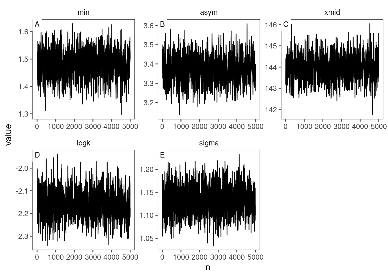
p_bayes_diagnostics$p_posterior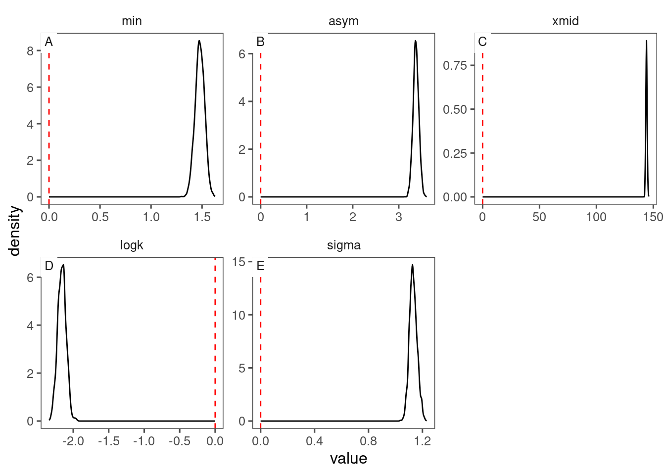
Make predictions.
df_pred <- calc_bayes_predict(
  data = dat %>%
    distinct(doy),
  df_MCMC = df_MCMC,
  version = 1
)
Plot predictions.
p_bayes_predict <- plot_bayes_predict(
  data = dat,
  data_predict = df_pred,
  vis_log = F
)

p_bayes_predict$p_original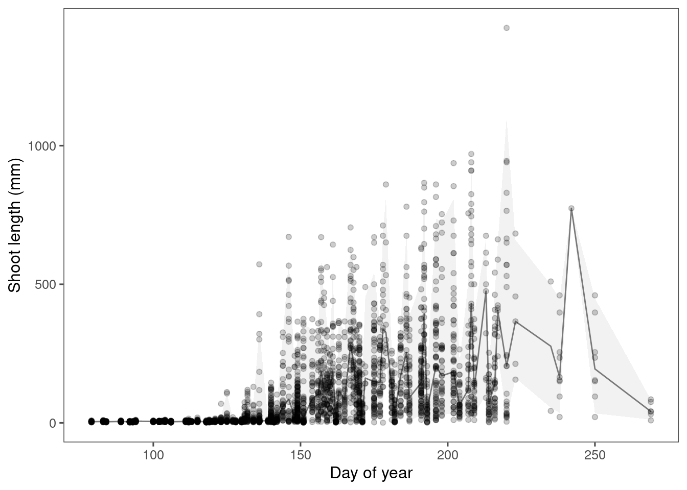
p_bayes_predict$p_overlay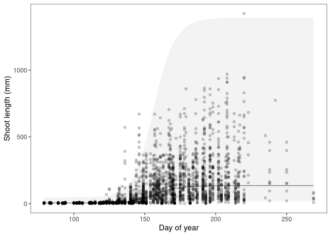
p_bayes_predict$p_accuracy
Plot predictions on log scale.
p_bayes_predict <- plot_bayes_predict(
  data = dat,
  data_predict = df_pred,
  vis_log = T
)

p_bayes_predict$p_original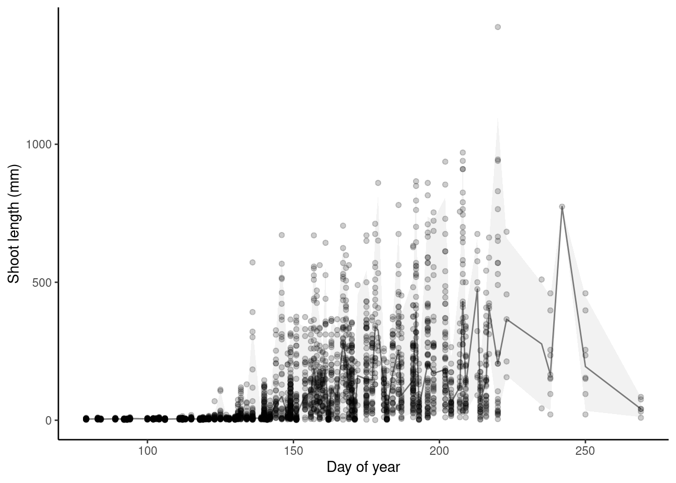
p_bayes_predict$p_overlay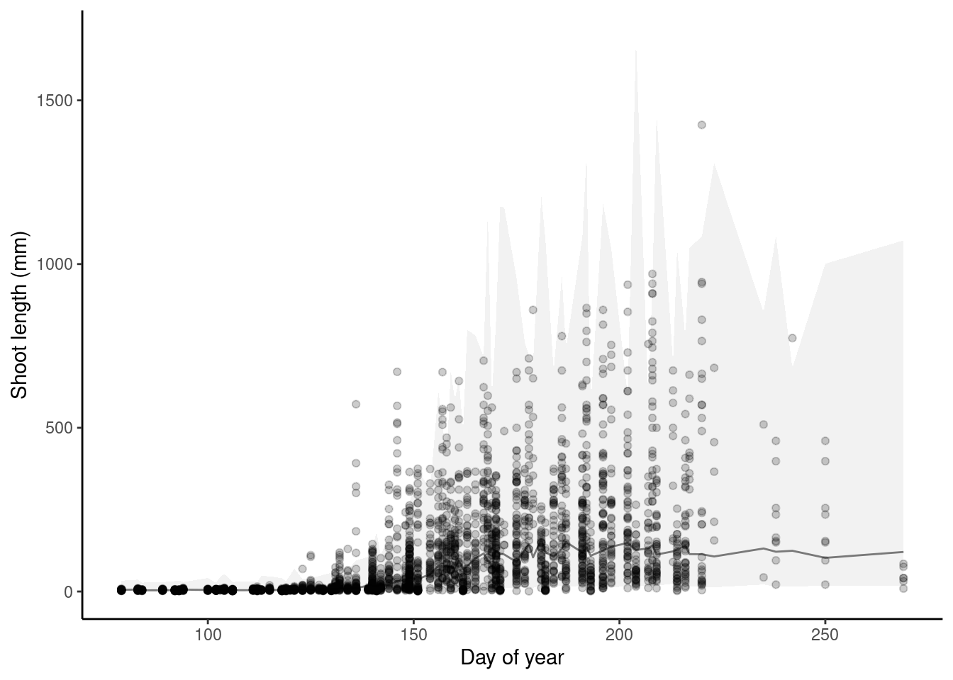
p_bayes_predict$p_accuracy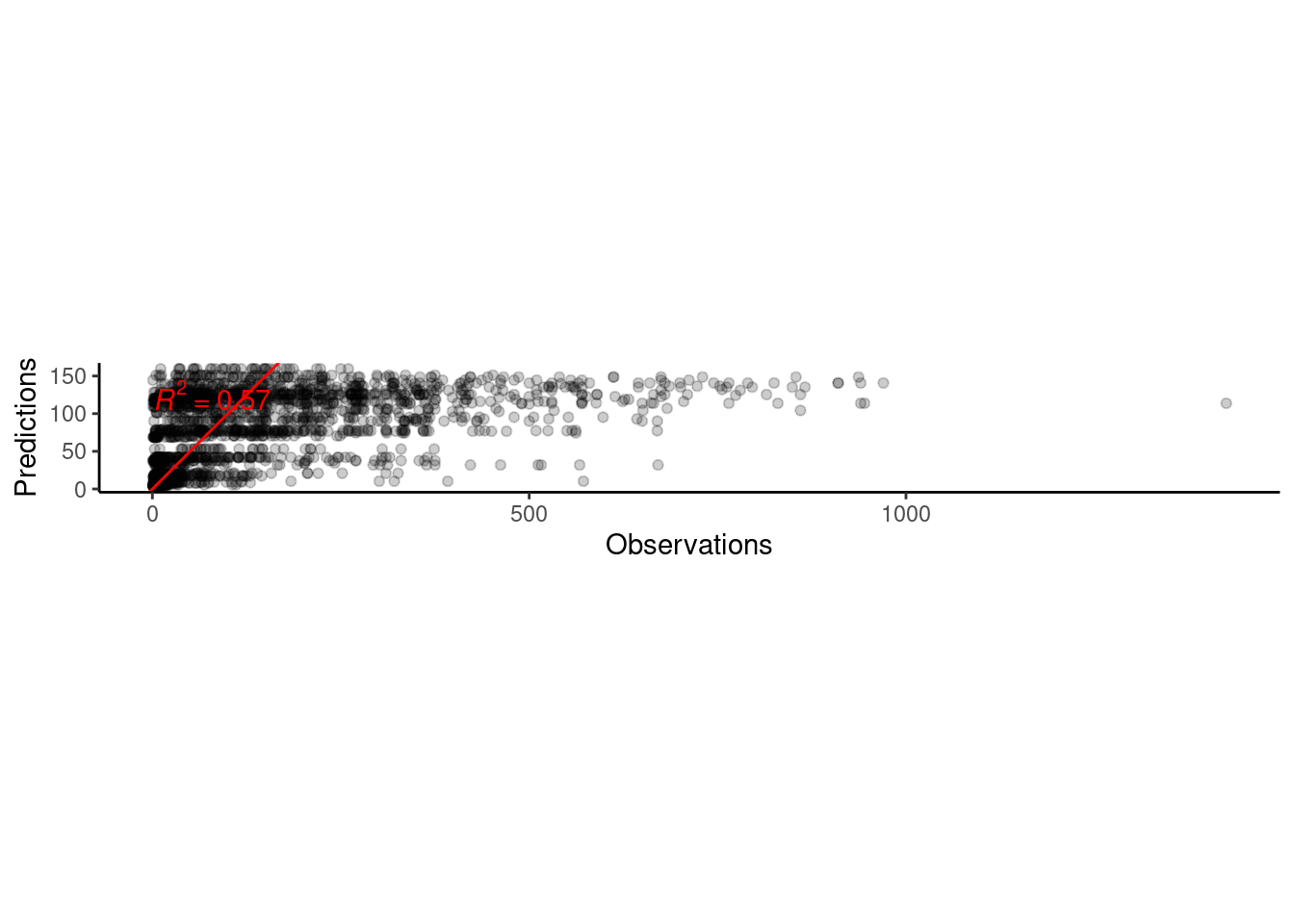
- Need to fix observational error to constrain shoot length >= 0. Fixed with lognormal distribution.
- Seem to be large differences between plots.
- Some outliers dominated because of changing sampling periods?
- Need to look at priors more closely.
Question about computation: What’s the best way to train with all 103408 data points from 4302 individuals?