Read in data from 2009 to 2020 in long format.
dat_phenophase## # A tibble: 4,116,485 × 16
## site canopy heat heat_name water water_name block plot species barcode
## <chr> <fct> <fct> <fct> <fct> <fct> <chr> <chr> <chr> <dbl>
## 1 cfc open _ ambient _ ambient d d1 abiba 1
## 2 cfc open _ ambient _ ambient d d1 abiba 1
## 3 cfc open _ ambient _ ambient d d1 abiba 1
## 4 cfc open _ ambient _ ambient d d1 abiba 1
## 5 cfc open _ ambient _ ambient d d1 abiba 1
## 6 cfc open _ ambient _ ambient d d1 abiba 1
## 7 cfc open _ ambient _ ambient d d1 abiba 1
## 8 cfc open _ ambient _ ambient d d1 abiba 1
## 9 cfc open _ ambient _ ambient d d1 abiba 1
## 10 cfc open _ ambient _ ambient d d1 abiba 1
## # ℹ 4,116,475 more rows
## # ℹ 6 more variables: cohort <dbl>, year <dbl>, doy <dbl>, phenophase <fct>,
## # status <dbl>, notes <chr>Question: What do I do about those with non-NA notes?
set.seed(1)
dat_phenophase %>%
  filter(!is.na(notes)) %>%
  group_by(notes) %>%
  select(plot, species, barcode, year, doy, phenophase, status, notes) %>%
  sample_n(1)
## # A tibble: 2,565 × 8
## # Groups: notes [2,565]
## plot species barcode year doy phenophase status notes
## <chr> <chr> <dbl> <dbl> <dbl> <fct> <dbl> <chr>
## 1 l7 rhaca 40843 2019 108 budbreak 0 "\""
## 2 k1 pinst 6844 2011 252 senescence 1 "\"\"dupliate deleted ba…
## 3 l2 poptr 40316 2020 310 budbreak 0 "\"not so much scenesced…
## 4 f3 acesa 2209 2011 137 oneleaf 0 "\"row added based on lh…
## 5 f6 fraal 38220 2018 121 leafdrop 0 "\"so close\""
## 6 j8 rhaca 39201 2019 108 mostleaf 0 "(formerly k13)"
## 7 h5 picgl 34593 2017 306 oneleaf 0 "(missing measurement? -…
## 8 k6 acesa 39967 2019 108 mostleaf 0 "(now j2)"
## 9 k7 betpa 40087 2019 108 mostleaf 0 "(now some l11)"
## 10 a3 picma 31319 2018 121 budbreak 0 "(picma?)"
## # ℹ 2,555 more rowsMultiple entries conflicting
dat_phenophase_full <- tidy_phenophase(distinct = F)
dat_phenophase_dup_group <- anti_join(dat_phenophase_full, dat_phenophase) %>%
  distinct(site, canopy, heat, heat_name, water, water_name, block, plot, species, barcode, cohort, year, doy, phenophase, notes)

dat_phenophase_dup <- dat_phenophase_full %>%
  right_join(dat_phenophase_dup_group)

dat_phenophase_dup %>%
  arrange(site, canopy, heat, heat_name, water, water_name, block, plot, species, barcode, cohort, year, doy, phenophase, notes) %>%
  select(plot, species, barcode, year, doy, phenophase, status, notes)
## # A tibble: 3,799 × 8
## plot species barcode year doy phenophase status notes
## <chr> <chr> <dbl> <dbl> <dbl> <fct> <dbl> <chr>
## 1 d5 queru 36443 2019 106 budbreak 0 <NA>
## 2 d5 queru 36443 2019 106 oneleaf 0 <NA>
## 3 d5 queru 36443 2019 106 mostleaf 0 <NA>
## 4 d5 queru 36443 2019 106 senescence 0 <NA>
## 5 d5 queru 36443 2019 106 leafdrop 0 <NA>
## 6 d5 queru 36443 2019 142 budbreak 1 <NA>
## 7 d5 queru 36443 2019 142 budbreak 0 <NA>
## 8 d5 queru 36443 2019 149 budbreak 1 <NA>
## 9 d5 queru 36443 2019 149 budbreak 0 <NA>
## 10 d5 queru 36443 2019 156 budbreak 1 <NA>
## # ℹ 3,789 more rowsTime of budbreak
dat_phenophase_time <- calc_phenophase_time(dat_phenophase)
p_phenophase_change <- plot_phenophase_change(dat_phenophase_time)
p_phenophase_change$budbreak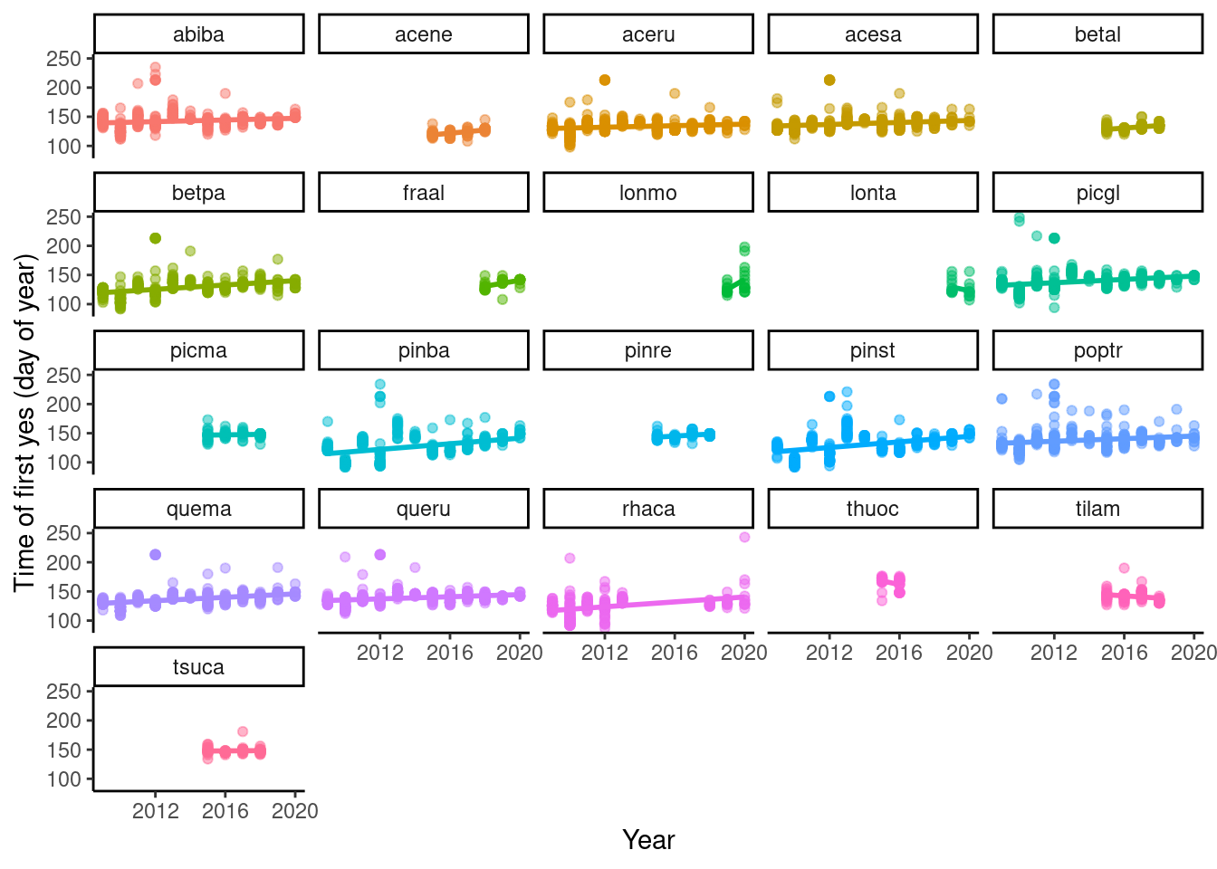
- 2012 seems to have more late outliers.
- If they were second flush, why were first flush never observed?
Example of outlier.
set.seed(1)
dat_phenophase_outlier <- dat_phenophase_time %>%
  filter(phenophase == "budbreak", doy > 180) %>%
  sample_n(1)
dat_phenophase_outlier %>% select(plot, species, barcode, year, phenophase, doy, notes)
## # A tibble: 1 × 7
## plot species barcode year phenophase doy notes
## <chr> <chr> <dbl> <dbl> <fct> <dbl> <chr>
## 1 k3 poptr 19823 2012 budbreak 213 <NA>dat_phenophase %>%
right_join(dat_phenophase_outlier %>% select(-doy)) %>%
filter(abs(doy - dat_phenophase_outlier$doy) <= 30) %>%
select(plot, species, barcode, year, doy, phenophase, status, notes)## # A tibble: 4 × 8
## plot species barcode year doy phenophase status notes
## <chr> <chr> <dbl> <dbl> <dbl> <fct> <dbl> <chr>
## 1 k3 poptr 19823 2012 213 budbreak 1 <NA>
## 2 k3 poptr 19823 2012 223 budbreak 1 <NA>
## 3 k3 poptr 19823 2012 235 budbreak 1 <NA>
## 4 k3 poptr 19823 2012 241 budbreak 0 <NA>Decided to remove outliers manually using time window.
dat_phenophase_time_clean <- calc_phenophase_time(dat_phenophase, remove_outlier = T)
dat_phenophase_clean <- tidy_phenophase(remove_outlier = T, dat_phenophase_time = dat_phenophase_time_clean)

setwd("phenologyb4warmed/")
usethis::use_data(dat_phenophase_time_clean, overwrite = T)
usethis::use_data(dat_phenophase_clean, overwrite = T)
setwd("..")
p_phenophase_change <- plot_phenophase_change(dat_phenophase_time_clean)
p_phenophase_change$budbreak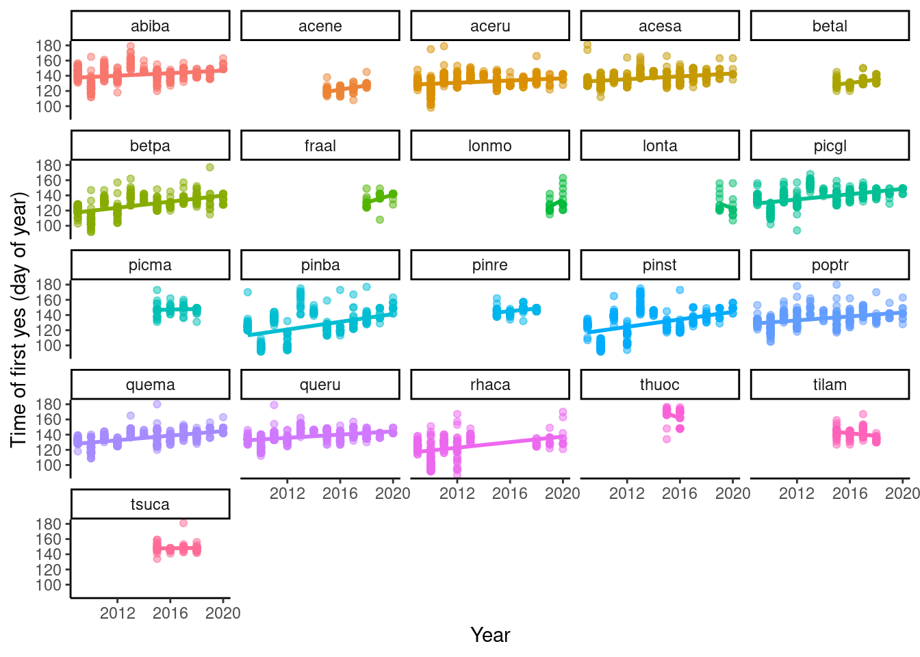 Better now.
Phenophases to ordinal data
dat_phenophase_ordinal <- tidy_phenophase_ordinal(dat_phenophase, season = "spring", keepfirst = F)
dat_phenophase_ordinal %>%
  select(plot, species, barcode, year, doy, budbreak, oneleaf, mostleaf, stage) %>%
  distinct(budbreak, oneleaf, mostleaf, stage, .keep_all = T)
## # A tibble: 8 × 9
## plot species barcode year doy budbreak oneleaf mostleaf stage
## <chr> <chr> <dbl> <dbl> <dbl> <dbl> <dbl> <dbl> <fct>
## 1 d1 abiba 1 2009 100 0 0 0 <NA>
## 2 d1 abiba 1 2009 138 1 0 0 budbreak
## 3 d1 abiba 1 2009 167 1 1 0 oneleaf
## 4 d1 abiba 1 2009 223 1 1 1 mostleaf
## 5 d4 abiba 372 2011 186 0 0 1 mostleaf
## 6 d4 abiba 16437 2013 185 0 1 0 oneleaf
## 7 d4 abiba 16437 2014 217 0 1 1 mostleaf
## 8 d4 acesa 396 2011 186 1 0 1 mostleaf- Does all No mean dormancy? (No.)
- If not, how to get dormancy? (Can assume that any time after we stopped surveys in the fall and before we started surveys in the spring is the dormancy time.)
- Yes for multiple categories? (Because some data are filled in, not observed. Use time of first yes only.)
Climate data
dat_climate_daily <- read_climate(option = "daily")
plot_climate(dat_climate_daily, plotoi = "a1")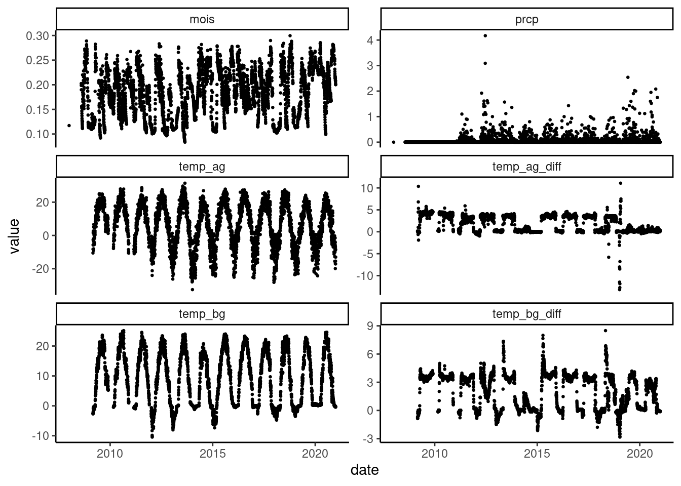
- Maximum hourly rainfall seems to be 2160 inches. Was there something wrong? (Now fixed.)
- Were the rainfall at reduced rainfall plots measured? (No. Now rainfall removal flag implemented.)
- Difference in aboveground temperature with ambient plot seems big in 2014 and 2019? (Not sure yet.)