Ordinal regression

Prepare ordinal data

Read in data from 2009 to 2020 in long format. Calculate time of first yes.

dat_phenophase_time <- calc_phenophase_time(dat_phenophase)

Convert binary (yes or no) data to ordinal (developmental stage) data. In this dataset, some individuals are scored as “budbreak” and “oneleaf” at the same time. I took the later stage. Note that I don’t have a category of “dormancy” because it can mean multiple things when scores for “budbreak” “oneleaf” and “mostleaf” are all zero.

dat_phenophase_ordinal <- tidy_phenophase_ordinal(dat_phenophase_time = dat_phenophase_time, season = "spring", keepfirst = T)

Table 1: Examples of ordinal stage determination.
budbreak	oneleaf	mostleaf	stage
1	0	0	budbreak
0	1	0	oneleaf
0	0	1	mostleaf
0	1	1	mostleaf
1	1	1	mostleaf
1	1	0	oneleaf

plot_phenophase_ordinal(dat_phenophase_ordinal)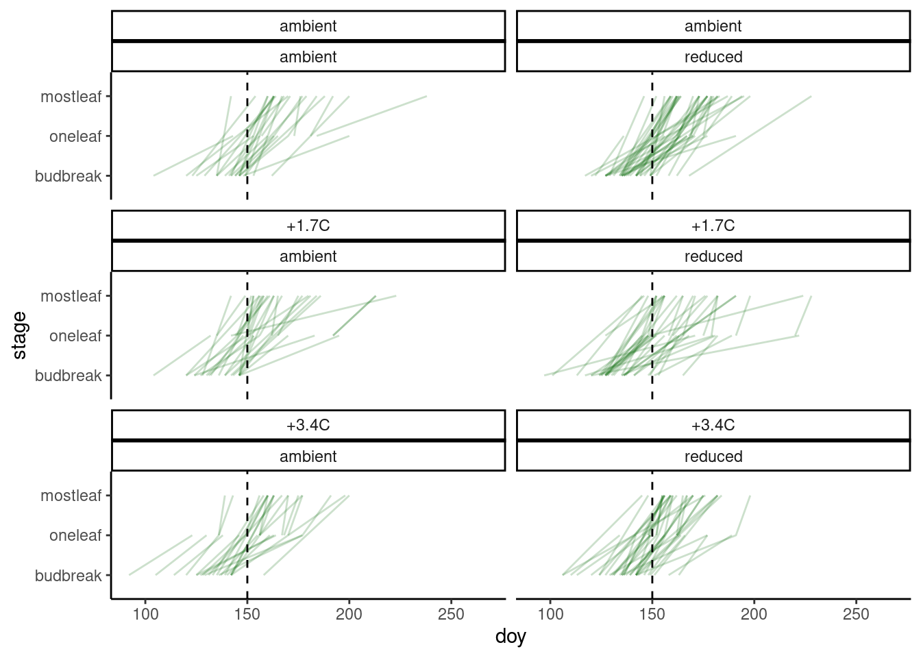

Figure 1: Changes in developmental stage over time of randomly selected individuals.

My simplest model:

\[ logit(P(S_i \le j))= \theta_j - \beta X_i \]

\[ X = [DOY, Heat+, Water-, Heat+ \times Water-, Heat+ \times DOY, Water- \times DOY] \]

\[ i = 1, ..., n \]

\[ j = budbreak, oneleaf, mostleaf \]

This is a model for the cumulative probability of the ith stage observation falling in the jth category or below, where i index all observations, j index the response categories, and _j is the intercept or threshold for the jth cumulative logit: logit(P(S_i <= j)).

I fit the model with the R package ordinal reference.

test_ordinal(dat_phenophase_ordinal %>% filter(species == "queru", canopy == "open", site == "cfc")) %>% summary()

## formula: stage ~ doy + heat + water + heat_water + heat_doy + water_doy
## data:    df
## 
##  link  threshold nobs logLik  AIC     niter max.grad cond.H 
##  logit flexible  1193 -814.79 1645.58 6(0)  8.76e-11 9.5e+07
## 
## Coefficients:
##            Estimate Std. Error z value Pr(>|z|)    
## doy         0.16736    0.01033  16.205  < 2e-16 ***
## heat        3.63363    0.98145   3.702 0.000214 ***
## water       1.31675    1.73531   0.759 0.447972    
## heat_water -0.11394    0.17484  -0.652 0.514627    
## heat_doy   -0.01961    0.00627  -3.127 0.001764 ** 
## water_doy  -0.01152    0.01062  -1.085 0.278045    
## ---
## Signif. codes:  0 '***' 0.001 '**' 0.01 '*' 0.05 '.' 0.1 ' ' 1
## 
## Threshold coefficients:
##                  Estimate Std. Error z value
## budbreak|oneleaf   25.233      1.620   15.57
## oneleaf|mostleaf   27.858      1.668   16.70

Results of ordinal regression interpreted as follows * Stage progresses over time in a spring * Warming leads to earlier development * Stronger warming leads to even earlier development * Rainfall reduction leads to earlier development * Interaction between warming and drying offsets advancement (not conclusive) * Warming slows down the pace of development (not conclusive) * Rainfall reduction slows down the pace of development (not conclusive)

Future directions

Questions * Model convergence issue? * What to do when categories are overlapping?

Short-term improvements * Fixed effects for site, canopy, species, background climate * Random effects for block * Choice of link function (currently logit) * Add “dormancy” category

Long-term developments * Changing the function for latent variable (currently linear)