Tidy up data
Read in data from 2009 to 2020. Convert data to long format.
dat_phenophase <- tidy_phenophase()

setwd("phenologyb4warmed/")
usethis::use_data(dat_phenophase, overwrite = T)
setwd("..")
I have stored processed data in the R package. Use it directly.
| site | canopy | heat | heat_name | water | water_name | block | plot | species | barcode | cohort | year | doy | phenophase | status | notes |
|---|---|---|---|---|---|---|---|---|---|---|---|---|---|---|---|
| cfc | open | _ | ambient | _ | ambient | d | d1 | abiba | 1 | 2008 | 2009 | 100 | budbreak | 0 | NA |
| cfc | open | _ | ambient | _ | ambient | d | d1 | abiba | 1 | 2008 | 2009 | 100 | oneleaf | 0 | NA |
| cfc | open | _ | ambient | _ | ambient | d | d1 | abiba | 1 | 2008 | 2009 | 100 | mostleaf | 0 | NA |
| cfc | open | _ | ambient | _ | ambient | d | d1 | abiba | 1 | 2008 | 2009 | 100 | senescence | 0 | NA |
| cfc | open | _ | ambient | _ | ambient | d | d1 | abiba | 1 | 2008 | 2009 | 100 | leafdrop | 0 | NA |
| cfc | open | _ | ambient | _ | ambient | d | d1 | abiba | 1 | 2008 | 2009 | 103 | budbreak | 0 | NA |
Calculate time of first yes for each site, canopy, treatment, block, plot, species, and phenophase combination.
dat_phenophase_time <- calc_phenophase_time(dat_phenophase)| site | canopy | heat | heat_name | water | water_name | block | plot | species | barcode | cohort | year | doy | phenophase | notes |
|---|---|---|---|---|---|---|---|---|---|---|---|---|---|---|
| cfc | open | _ | ambient | _ | ambient | d | d1 | abiba | 1 | 2008 | 2009 | 138 | budbreak | NA |
| cfc | open | _ | ambient | _ | ambient | d | d1 | abiba | 1 | 2008 | 2009 | 167 | oneleaf | NA |
| cfc | open | _ | ambient | _ | ambient | d | d1 | abiba | 1 | 2008 | 2009 | 223 | mostleaf | NA |
| cfc | open | _ | ambient | _ | ambient | d | d1 | abiba | 1 | 2008 | 2009 | 261 | senescence | NA |
| cfc | open | _ | ambient | _ | ambient | d | d1 | abiba | 1 | 2008 | 2009 | 282 | leafdrop | NA |
| cfc | open | _ | ambient | _ | ambient | d | d1 | abiba | 11 | 2008 | 2009 | 138 | budbreak | NA |
Change in phenophase time in ambient plots over years
p_phenophase_change <- plot_phenophase_change(dat_phenophase_time)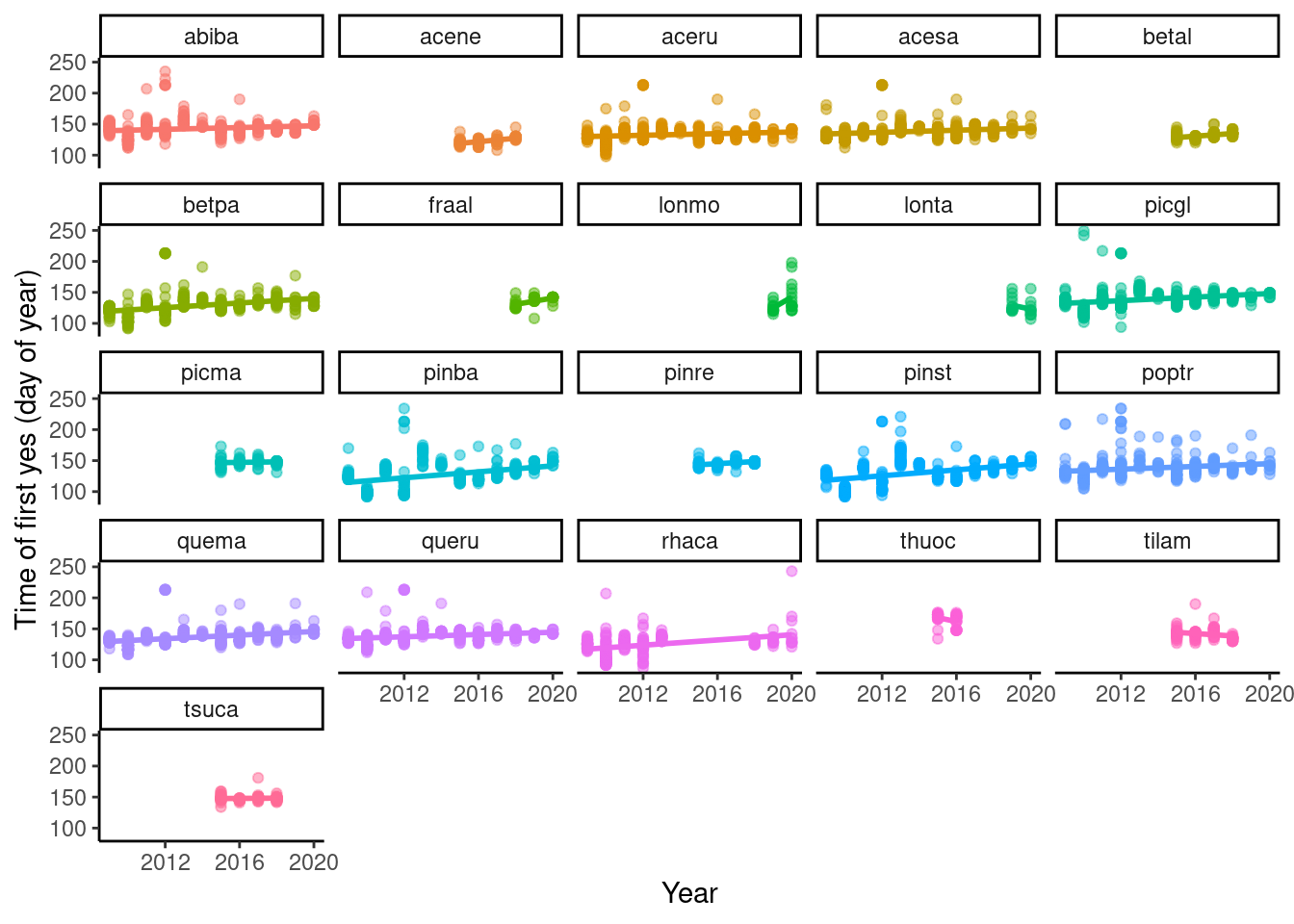
Figure 1: Change in budbreak time in ambient plot over years.
- Overall delay in time of budbreak. Check climate trend in the area.
- First five years seem to have more outliers. Check if I used the correctly cleaned data.
Difference in phenophase time induced by treatments
Using average time of first yes in ambient plots in each site, canopy, block, species, phenophase, and year as baseline, I calculate the difference between each individual’s time to the baseline. This difference in phenophase time represent the effect of treatments.
dat_phenophase_diff <- calc_phenophase_diff(dat_phenophase_time)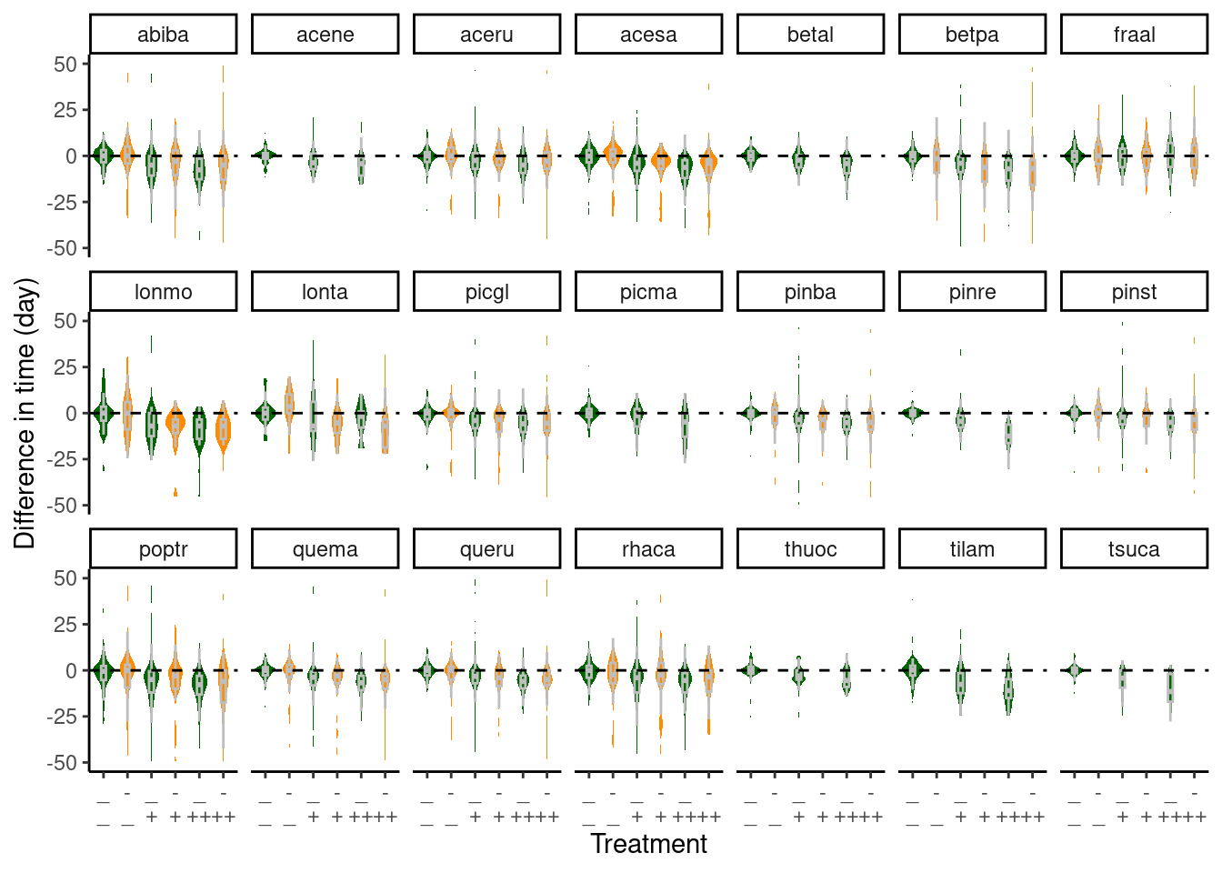
Figure 2: Difference in individuals’ budbreak time compared to average time ambient plots. Green - ambient rainfall; Orange - reduced rainfall.
- Warming advanced budbreak in both ambient and reduced rainfall.
- Reduced rainfall dampened the effect of warming.
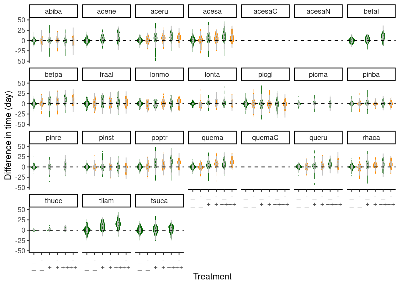
Figure 3: Difference in individuals’ senescence time compared to average time ambient plots. Green - ambient rainfall; Orange - reduced rainfall.
- For most deciduous species, warming delayed senescence in both ambient and reduced rainfall.
- Reduced rainfall may have dampened the effect of warming, but more tests need to be done.
- Evergreen trees’ senescence did not respond much to warming or drying.
Relationship between effect size and baseline
I try to reproduce Montgomery et al. (2020) in PNAS (paper). I first pool individuals in plots together to estimate the time of phenophase for each site, canopy, treatment, block, species, phenophase, and year. I compare the phenophase time to the baseline in ambient plots again to get a difference in phenophase time.
dat_phenophase_time_summ <- summ_phenophase_time(dat_phenophase_time)
dat_phenophase_diff_summ <- calc_phenophase_diff(dat_phenophase_time_summ)
I then look at if the effect of warming treatment differ between warm and early years and cold and later years. Instead of using temperature on the x-axis, I use the baseline phenophase time in ambient plots on the x-axis, because I don’t have environmental data yet.
In Montgomery et al. (2020), they used a community-level effect size by averaging 10 species’ effect size. I try to do the same, using data in 2009-2013.
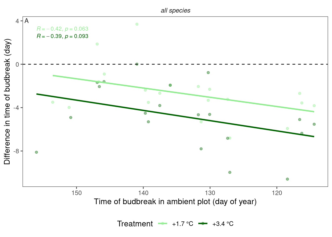
Figure 4: Relationship between phenology in ambient plot and average effect of warming treatment on budbreak time, using data from 2009-2013.
- Effect of warming is stronger in early years compared to late years.
- Relationship only marginally significant, probably because phenology im ambient plot is not a perfect proxy for temperature.
- Effect of 3.4°C warming was roughly twice of that of 1.7°C.
I extend the same analysis to 2009-2020.
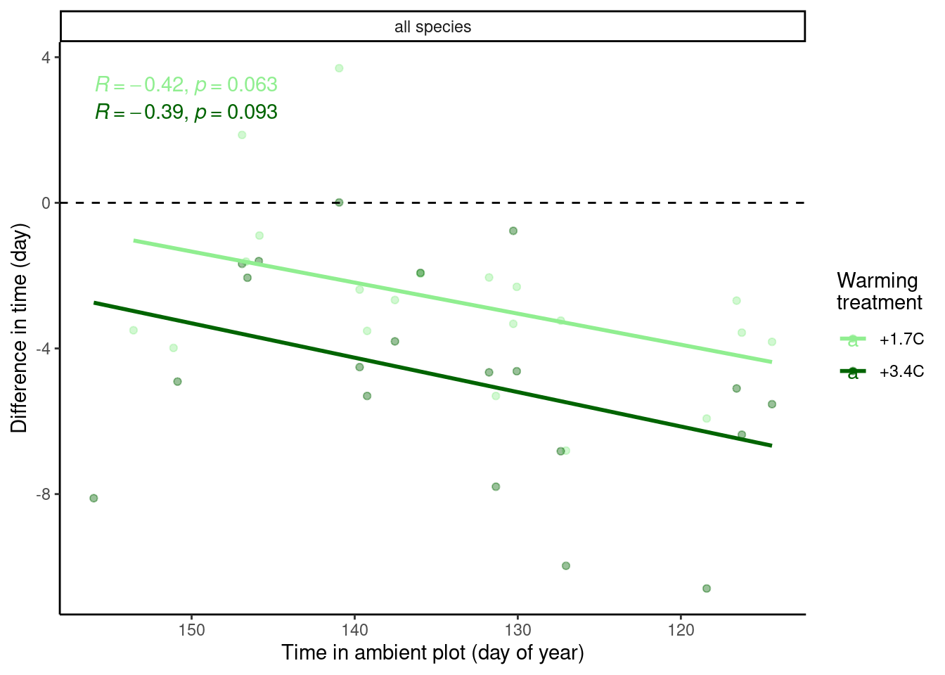
Figure 5: Relationship between phenology in ambient plot and average effect of warming treatment on budbreak time, using data from 2009-2020.
- Relationship still holds qualitatively.
- Less significant probably because in the first five years, there were some extremely early or late years, but later on we saw some intermediate years, with large variations in treatment effect.
I’m not too sure if pooling all species is fair, so I look at the relationship by species.
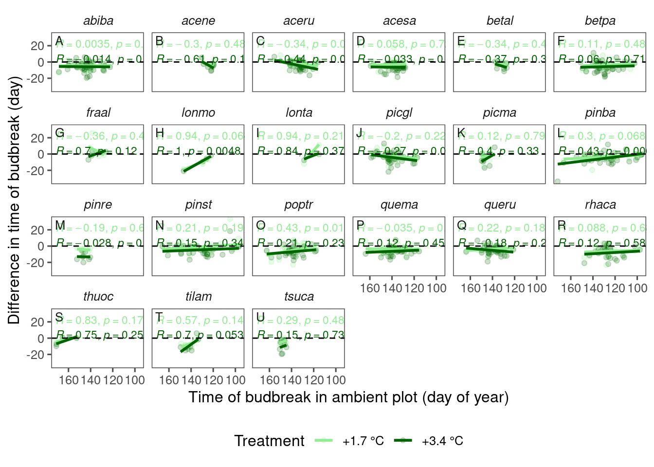
Figure 6: Relationship between phenology in ambient plot and species-specific effect of warming treatment on budbreak time, using data from 2009-2013.
- The relationship between block-level effect and baseline may have been driven by some species such as red maple, white spruce, and red oak.
- Some species such as trembling aspen and white pine showed the opposite relationship.